classbound

classbound is an R package for exploring and comparing classification decision boundaries. It provides a unified interface for fitting classifiers, computing 2D boundary grids, and visualizing how different models partition the feature space.

What you can do with classbound:

Visualize decision boundaries for any R classifier
Compare multiple classifiers side by side
Handle high-dimensional data via 2D slicing or projection (PCA, tourr)
View probability surfaces for classifiers that provide them
Explore data interactively using the built-in Shiny app (explorapp())
Integrate natively with tidymodels workflows

Full documentation: https://natydasilva.github.io/classbound/

Installation

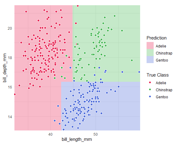
devtools::install_github("natydasilva/classbound")

Quick start

One-step wrapper

classbound() fits a model, computes its decision boundary, and plots the result in a single call.

library(classbound)
library(palmerpenguins)

penguins <- na.omit(palmerpenguins::penguins[
  ,
  c("species", "bill_length_mm", "bill_depth_mm")
])

classbound(
  data       = penguins,
  formula    = species ~ bill_length_mm + bill_depth_mm,
  classifier = rpart::rpart
)

Modular pipeline

For full control, use the three-step pipeline:

# 1. Fit
model <- fit_model(penguins, species ~ bill_length_mm + bill_depth_mm, rpart::rpart)

# 2. Compute boundary
model <- boundary_compute(model)

# 3. Plot
plot_boundary(
  model,
  obs_data   = penguins,
  x_col      = "bill_length_mm",
  y_col      = "bill_depth_mm",
  true_label = "species"
)

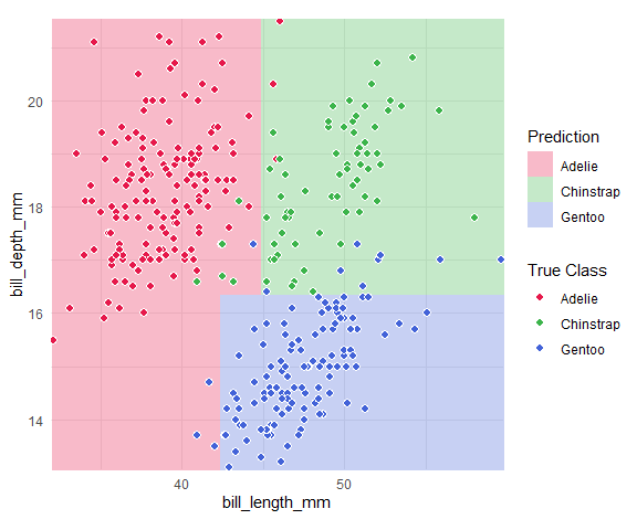
boundary_compute() returns the model with the grid attached, so you can replot with different settings without refitting.

Interactive workflow

Launch the built-in Shiny application for point-and-click exploration:

# Start with your own dataset
explorapp(data = penguins, target_col = "species")

# Or start empty and simulate/draw data
explorapp()

In explorapp() you can: - Import real data or simulate synthetic datasets - Draw classification data by hand - Fit and compare multiple classifiers simultaneously - Switch between 2D Slice and Projection views for high-dimensional data - Inject outliers and observe how boundaries shift - Inspect probability surfaces (for supported classifiers) - Export data, models, plots, and a reproduce script

Two main workflows

Interactive

Use explorapp() to:

Choose or create data
Choose models
Explore decision boundaries
Navigate, zoom, and draw
Compare models and export results

Programmatic

Use the core Classbound functions directly:

fit_model()
boundary_compute()
plot_boundary()

High-dimensional data

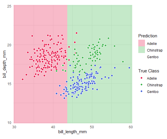
When a model is trained on more than two features, boundary_compute() supports:

2D Slice: two features are plotted; other features are fixed at their median/mode.

penguins3 <- na.omit(palmerpenguins::penguins[
  ,
  c("species", "bill_length_mm", "bill_depth_mm", "flipper_length_mm")
])

m3 <- fit_model(penguins3, species ~ ., rpart::rpart)
m3_slice <- boundary_compute(m3,
  feature_range = list(bill_length_mm = c(30, 60), bill_depth_mm = c(10, 25)),
  resolution = 60
)

plot_boundary(m3_slice,
  obs_data = penguins3,
  x_col = "bill_length_mm", y_col = "bill_depth_mm",
  true_label = "species"
)

Projection: all features are combined into two projected axes (e.g., PCA).

feat_cols <- c("bill_length_mm", "bill_depth_mm", "flipper_length_mm")
pca <- prcomp(penguins3[, feat_cols], scale. = TRUE)
basis <- pca$rotation[, 1:2]

x_std <- scale(penguins3[, feat_cols], center = pca$center, scale = pca$scale)
z_mat <- x_std %*% basis

m3_proj <- boundary_compute(m3,
  feature_range = list(
    PC1 = range(z_mat[, 1]) + c(-0.5, 0.5),
    PC2 = range(z_mat[, 2]) + c(-0.5, 0.5)
  ),
  resolution = 60,
  projection = list(basis = basis, center = pca$center, scale = pca$scale)
)

plot_boundary(m3_proj,
  obs_data = penguins3,
  x_col = "PC1", y_col = "PC2", true_label = "species"
)

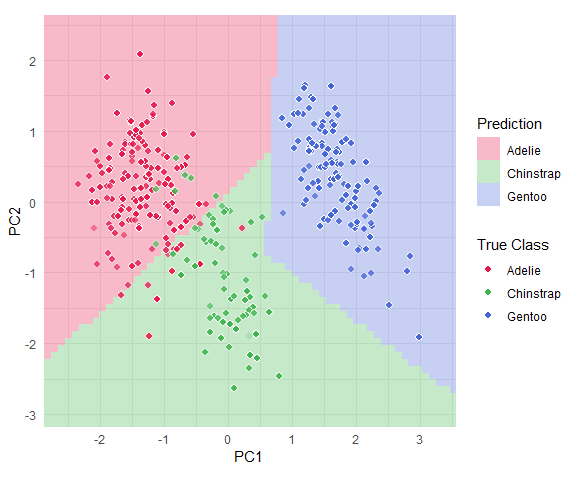
See the high-dimensional guide for a full explanation.

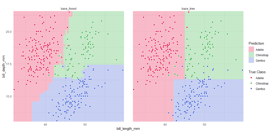
Multi-model comparison with tidymodels

library(parsnip)
library(workflowsets)

spec_tree <- decision_tree(mode = "classification") |> set_engine("rpart")
spec_rf <- rand_forest(mode = "classification") |> set_engine("randomForest")

wf_set <- workflow_set(
  preproc = list(base = species ~ bill_length_mm + bill_depth_mm),
  models  = list(tree = spec_tree, forest = spec_rf)
)

bounds <- boundary_workflow_set(wf_set,
  data = penguins,
  response = "species", resolution = 60
)

plot_boundary(bounds,
  obs_data = penguins,
  x_col = "bill_length_mm", y_col = "bill_depth_mm",
  true_label = "species"
)

Documentation

Resource	Link
Getting Started	getting-started
High-Dimensional	high-dimensional
tidymodels	tidymodels-workflow
tourr	tourr-workflow
Explorapp Guide	explorapp-guide
Custom Adapters	custom_adapters
Reference	Function Reference

mirror server hosted at Truenetwork, Russian Federation.