


The aim of the prcbench package is to provide a testing
workbench for evaluating precision-recall curves under various
conditions. It contains integrated interfaces for the following seven
tools. It also contains predefined test data sets.
| Tool | Language | Link |
|---|---|---|
| precrec | R | Tool web site, CRAN |
| ROCR | R | Tool web site, CRAN |
| PRROC | R | CRAN |
| AUCCalculator | Java | Tool web site |
| PerfMeas | R | CRAN |
| yardstick | R | Tool web site, CRAN |
| sklearn | Python | Tool web site |
The sklearn tool uses a standalone Python module bundled
with prcbench and derived from the scikit-learn source, so
scikit-learn itself is not required. It does need the
reticulate package, Python and numpy. Without
them it returns a flat dummy curve instead of raising an error, so the
predefined tool sets that contain it stay usable.
Timings of sklearn are not comparable with those
of the R tools. Every call crosses the R/Python boundary and
converts the input and output vectors, and that overhead is counted as
part of the measurement. It often dominates the curve calculation itself
on small test sets. Use run_benchmark to compare the R
tools with each other, and read the sklearn row as the cost
of calling Python from R rather than as the speed of the scikit-learn
algorithm. Curve accuracy from run_evalcurve is
unaffected.
Disclaimer: prcbench was originally
develop to help our precrec library in
order to provide fast and accurate calculations of precision-recall
curves with extra functionality.
prcbench uses pre-defined test sets to help evaluate the
accuracy of precision-recall curves.
create_toolset: creates objects of different tools for
testing (7 different tools)create_testset: selects pre-defined data sets (c1, c2,
and c3)run_evalcurve: evaluates the selected tools on the
simulation dataautoplot: shows the results with ggplot2
and patchwork## Load library
library(prcbench)
## Plot base points and the result of 7 tools on pre-defined test sets (c1, c2, and c3)
toolset <- create_toolset(c(
"precrec", "ROCR", "AUCCalculator", "PerfMeas", "PRROC", "yardstick", "sklearn"
))
testset <- create_testset("curve", c("c1", "c2", "c3"))
scores1 <- run_evalcurve(testset, toolset)
autoplot(scores1, ncol = 4, nrow = 2)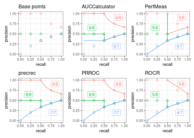
prcbench helps create simulation data to measure
computational times of creating precision-recall curves.
create_toolset: creates objects of different tools for
testingcreate_testset: creates simulation datarun_benchmark: evaluates the selected tools on the
simulation data## Load library
library(prcbench)
## Run benchmark for auc7 (7 tools) on four balanced test sets, from b100
## (50 positives and 50 negatives) up to b100000 (50,000 and 50,000)
toolset <- create_toolset(set_names = "auc7")
testset <- create_testset("bench", c("b100", "b1000", "b10000", "b100000"))
res <- run_benchmark(testset, toolset, unit = "s")
print(res)Test sets for benchmarking are named by a prefix followed by a total
size. The prefix b means balanced, half positives and half
negatives, and i means imbalanced, a quarter positives. The
number is how many data points the set holds, so b100 is 50
positives and 50 negatives, and b100000 is 50,000 of
each.
The table holds the mean running time in seconds. Each column is one
balanced test set, headed by the number of data points it contains.
These numbers are recorded by
data-raw/run_readme_benchmark.R and read from
data-raw/readme_benchmark.csv, not measured while this page
is knitted. Timing the tools on every knit made the numbers drift with
whatever else the machine was doing, so the benchmark is re-run
deliberately, when a wrapped tool changes or when there is a performance
change worth showing.
| Tool | 100 | 1,000 | 10,000 | 100,000 |
|---|---|---|---|---|
| AUCCalculator | 0.00307 | 0.011 | 0.0977 | 5.96 |
| PerfMeas | 0.000126 | 0.000243 | 0.00155 | 0.0147 |
| precrec | 0.0062 | 0.00625 | 0.00786 | 0.029 |
| PRROC | 0.000256 | 0.000489 | 0.00306 | 0.0359 |
| ROCR | 0.00206 | 0.00383 | 0.0211 | 0.238 |
| sklearn | 0.000519 | 0.000791 | 0.0036 | 0.0367 |
| yardstick | 0.00189 | 0.0025 | 0.00826 | 0.0705 |
Recorded on 2026-09-25 with R version 4.6.1 (2026-06-24) on
x86_64-pc-linux-gnu, 5 iterations per tool, using precrec
0.24.0, ROCR 1.0.12, PRROC 1.4, yardstick 1.4.0.
The sklearn row of the table includes the R/Python
conversion overhead, so it measures the round trip rather than the
scikit-learn algorithm. See the note above.
Introduction
to prcbench: a package vignette that contains the descriptions of
the functions with several useful examples. View the vignette with
vignette("introduction", package = "prcbench") in
R.
Help
pages: all the functions including the S3 generics have their own
help pages with plenty of examples. View the main help page with
help(package = "prcbench") in R.
install.packages("prcbench")AUCCalculator requires a Java runtime environment (>=
6) if AUCCalculator needs to be evaluated.
You can install a development version of prcbench from
our GitHub
repository.
devtools::install_github("evalclass/prcbench")Make sure you have a working development environment.
Windows: Install Rtools (available on the CRAN website).
Mac: Install Xcode from the Mac App Store.
Linux: Install a compiler and various development libraries (details vary across different flavors of Linux).
Install devtools from CRAN with
install.packages("devtools").
Install prcbench from the GitHub repository with
devtools::install_github("evalclass/prcbench").
microbenchmark
does not work on some OSs. prcbench uses
system.time when microbenchmark is not
available.
sudo R CMD javareconfPrecrec: fast and accurate precision-recall and ROC curve calculations in R
Takaya Saito; Marc Rehmsmeier
Bioinformatics 2017; 33 (1): 145-147.
doi: 10.1093/bioinformatics/btw570
Classifier evaluation with imbalanced datasets: our web site that contains several pages with useful tips for performance evaluation on binary classifiers.
The Precision-Recall Plot Is More Informative than the ROC Plot When Evaluating Binary Classifiers on Imbalanced Datasets: our paper that summarized potential pitfalls of ROC plots with imbalanced datasets and advantages of using precision-recall plots instead.