BayesSurvive

This is a R/Rcpp package BayesSurvive for Bayesian survival models with graph-structured selection priors for sparse identification of high-dimensional features predictive of survival (Hermansen et al., 2025; Madjar et al., 2021) (see the three models of the first column in the table below) and its extensions with the use of a fixed graph via a Markov Random Field (MRF) prior for capturing known structure of high-dimensional features (see the three models of the second column in the table below), e.g. disease-specific pathways from the Kyoto Encyclopedia of Genes and Genomes (KEGG) database.

Installation

Install the latest released version from CRAN

install.packages("BayesSurvive")

Install the latest development version from GitHub

#install.packages("remotes")
remotes::install_github("ocbe-uio/BayesSurvive")

Examples

Simulate data

library("BayesSurvive")
# Load the example dataset
data("simData", package = "BayesSurvive")
dataset = list("X" = simData[[1]]$X, 
               "t" = simData[[1]]$time,
               "di" = simData[[1]]$status)

Run a Bayesian Cox model

## Initial value: null model without covariates
initial = list("gamma.ini" = rep(0, ncol(dataset$X)))
# Prior parameters
hyperparPooled = list(
  "c0"     = 2,                      # prior of baseline hazard
  "tau"    = 0.0375,                 # sd (spike) for coefficient prior
  "cb"     = 20,                     # sd (slab) for coefficient prior
  "pi.ga"  = 0.02,                   # prior variable selection probability for standard Cox models
  "a"      = -4,                     # hyperparameter in MRF prior
  "b"      = 0.1,                    # hyperparameter in MRF prior
  "G"      = simData$G               # hyperparameter in MRF prior
)   

## run Bayesian Cox with graph-structured priors
set.seed(123)
fit <- BayesSurvive(survObj = dataset, model.type = "Pooled", MRF.G = TRUE, 
                    hyperpar = hyperparPooled, initial = initial, 
                    nIter = 200, burnin = 100)

## show posterior mean of coefficients and 95% credible intervals
library("GGally")
plot(fit) + 
  coord_flip() + 
  theme(axis.text.x = element_text(angle = 90, size = 7))

Show the index of selected variables by controlling Bayesian false discovery rate (FDR) at the level \(\alpha = 0.05\)

which( VS(fit, method = "FDR", threshold = 0.05) )

#[1]   1   2   3   4   5   6   7   8   9  10  11  12  13  14  15 128

Plot time-dependent Brier scores

The function BayesSurvive::plotBrier() can show the time-dependent Brier scores based on posterior mean of coefficients or Bayesian model averaging.

plotBrier(fit, survObj.new = dataset)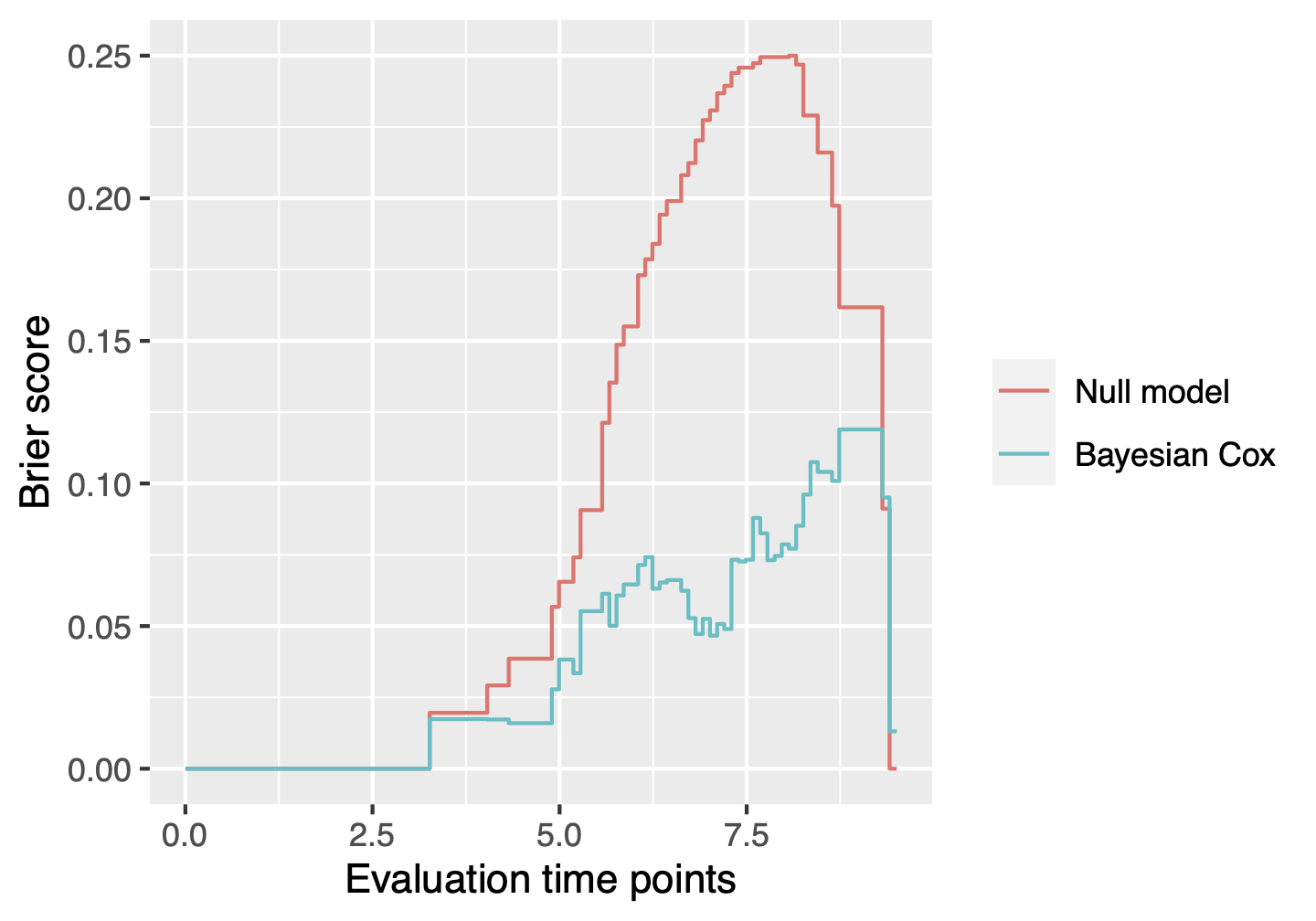

We can also use the function BayesSurvive::predict() to obtain the Brier score at time 8.5, the integrated Brier score (IBS) from time 0 to 8.5 and the index of prediction accuracy (IPA).

predict(fit, survObj.new = dataset, times = 8.5)

##               Brier(t=8.5) IBS(t:0~8.5) IPA(t=8.5)
## Null.model      0.2290318   0.08185316  0.0000000
## Bayesian.Cox    0.1037802   0.03020026  0.5468741

Predict survival probabilities and cumulative hazards

The function BayesSurvive::predict() can estimate the survival probabilities and cumulative hazards.

predict(fit, survObj.new = dataset, type = c("cumhazard", "survival"))

#        observation times cumhazard  survival
##              <int> <num>     <num>     <num>
##     1:           1   3.3  1.04e-04 1.00e+00
##     2:           2   3.3  3.88e-01 6.78e-01
##     3:           3   3.3  1.90e-06 1.00e+00
##     4:           4   3.3  1.94e-03 9.98e-01
##     5:           5   3.3  4.08e-04 1.00e+00
##    ---                                     
##  9996:          96   9.5  1.40e+01 8.21e-07
##  9997:          97   9.5  8.25e+01 1.45e-36
##  9998:          98   9.5  5.37e-01 5.85e-01
##  9999:          99   9.5  2.00e+00 1.35e-01
## 10000:         100   9.5  3.58e+00 2.79e-02

Run a ‘Pooled’ Bayesian Cox model with graphical learning

hyperparPooled <- append(hyperparPooled, list("lambda" = 3, "nu0" = 0.05, "nu1" = 5))
fit2 <- BayesSurvive(survObj = list(dataset), model.type = "Pooled", MRF.G = FALSE,
                     hyperpar = hyperparPooled, initial = initial, nIter = 10)

Run a Bayesian Cox model with subgroups using fixed graph

# specify a fixed joint graph between two subgroups
hyperparPooled$G <- Matrix::bdiag(simData$G, simData$G)
dataset2 <- simData[1:2]
dataset2 <- lapply(dataset2, setNames, c("X", "t", "di", "X.unsc", "trueB"))
fit3 <- BayesSurvive(survObj = dataset2, 
                     hyperpar = hyperparPooled, initial = initial, 
                     model.type="CoxBVSSL", MRF.G = TRUE, 
                     nIter = 10, burnin = 5)

Run a Bayesian Cox model with subgroups using graphical learning

fit4 <- BayesSurvive(survObj = dataset2, 
                     hyperpar = hyperparPooled, initial = initial, 
                     model.type="CoxBVSSL", MRF.G = FALSE, 
                     nIter = 3, burnin = 0)

References

Tobias Østmo Hermansen, Manuela Zucknick, Zhi Zhao (2025). Bayesian Cox model with graph-structured variable selection priors for multi-omics biomarker identification. arXiv. DOI: arXiv.2503.13078.

Katrin Madjar, Manuela Zucknick, Katja Ickstadt, Jörg Rahnenführer (2021). Combining heterogeneous subgroups with graph‐structured variable selection priors for Cox regression. BMC Bioinformatics, 22(1):586. DOI: 10.1186/s12859-021-04483-z.

mirror server hosted at Truenetwork, Russian Federation.