README

The package bayesRecon implements several methods for probabilistic reconciliation of hierarchical time series forecasts.

News

:boom: [2024-05-29] Added reconc_MixCond and reconc_TDcond and the vignette “Reconciliation of M5 hierarchy with mixed-type forecasts”.

:boom: [2023-12-19] Added the vignette “Properties of the reconciled distribution via conditioning”.

:boom: [2023-08-23] Added the vignette “Probabilistic Reconciliation via Conditioning with bayesRecon”. Added the schaferStrimmer_cov function.

Installation

install.packages("bayesRecon", dependencies = TRUE)

# install.packages("devtools")
devtools::install_github("IDSIA/bayesRecon", build_vignettes = TRUE, dependencies = TRUE)

Usage

Let us consider the minimal temporal hierarchy in the figure, where the bottom variables are the two 6-monthly forecasts and the upper variable is the yearly forecast. We denote the variables for the two semesters and the year by \(S_1, S_2, Y\) respectively.

The hierarchy is described by the aggregation matrix A, which can be obtained using the function get_reconc_matrices.

library(bayesRecon)

rec_mat <- get_reconc_matrices(agg_levels = c(1, 2), h = 2)
A <- rec_mat$A
print(A)
#>      [,1] [,2]
#> [1,]    1    1

Example 1: Poisson base forecasts

We assume that the base forecasts are Poisson distributed, with parameters given by \(\lambda_{Y} = 9\), \(\lambda_{S_1} = 2\), and \(\lambda_{S_2} = 4\).

lambdaS1 <- 2
lambdaS2 <- 4
lambdaY <- 9
lambdas <- c(lambdaY, lambdaS1, lambdaS2)
n_tot = length(lambdas)

base_forecasts = list()
for (i in 1:n_tot) {
  base_forecasts[[i]] = list(lambda = lambdas[i])
}

We recommend using the BUIS algorithm (Zambon et al., 2024) to sample from the reconciled distribution.

buis <- reconc_BUIS(
  A,
  base_forecasts,
  in_type = "params",
  distr = "poisson",
  num_samples = 100000,
  seed = 42
)

samples_buis <- buis$reconciled_samples

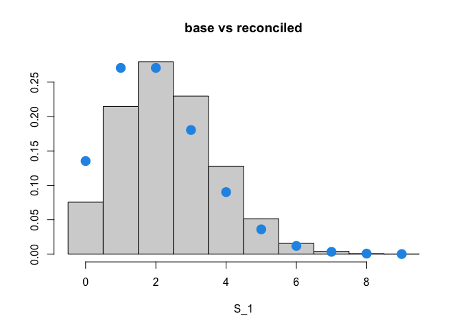
Since there is a positive incoherence in the forecasts (\(\lambda_Y > \lambda_{S_1}+\lambda_{S_2}\)), the mean of the bottom reconciled forecast increases. We show below this behavior for \(S_1\).

reconciled_forecast_S1 <- buis$bottom_reconciled_samples[1,]
range_forecats <- range(reconciled_forecast_S1)
hist(
  reconciled_forecast_S1,
  breaks = seq(range_forecats[1] - 0.5, range_forecats[2] + 0.5),
  freq = F,
  xlab = "S_1",
  ylab = NULL,
  main = "base vs reconciled"
)
points(
  seq(range_forecats[1], range_forecats[2]),
  stats::dpois(seq(range_forecats[1], range_forecats[2]), lambda =
                 lambdaS1),
  pch = 16,
  col = 4,
  cex = 2
)

The blue circles represent the probability mass function of a Poisson with parameter \(\lambda_{S_1}\) plotted on top of the histogram of the reconciled bottom forecasts for \(S_1\). Note how the histogram is shifted to the right.

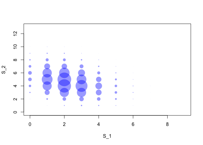
Moreover, while the base bottom forecast were assumed independent, the operation of reconciliation introduced a negative correlation between \(S_1\) and \(S_2\). We can visualize it with the plot below which shows the empirical correlations between the reconciled samples of \(S_1\) and the reconciled samples of \(S_2\).

AA <-
  xyTable(buis$bottom_reconciled_samples[1, ],
          buis$bottom_reconciled_samples[2, ])
plot(
  AA$x ,
  AA$y ,
  cex = AA$number * 0.001  ,
  pch = 16 ,
  col = rgb(0, 0, 1, 0.4) ,
  xlab = "S_1" ,
  ylab = "S_2" ,
  xlim = range(buis$bottom_reconciled_samples[1, ]) ,
  ylim = range(buis$bottom_reconciled_samples[2, ])
)

We also provide a function for sampling using Markov Chain Monte Carlo (Corani et al., 2023).

mcmc = reconc_MCMC(
  A,
  base_forecasts,
  distr = "poisson",
  num_samples = 30000,
  seed = 42
)

samples_mcmc <- mcmc$reconciled_samples

Example 2: Gaussian base forecasts

We now assume that the base forecasts are Gaussian distributed, with parameters given by

muS1 <- 2
muS2 <- 4
muY <- 9
mus <- c(muY, muS1, muS2)

sigmaS1 <- 2
sigmaS2 <- 2
sigmaY <- 3
sigmas <- c(sigmaY, sigmaS1, sigmaS2)

base_forecasts = list()
for (i in 1:n_tot) {
  base_forecasts[[i]] = list(mean = mus[[i]], sd = sigmas[[i]])
}

buis <- reconc_BUIS(
  A,
  base_forecasts,
  in_type = "params",
  distr = "gaussian",
  num_samples = 100000,
  seed = 42
)
samples_buis <- buis$reconciled_samples
buis_means <- rowMeans(samples_buis)

If the base forecasts are Gaussian, the reconciled distribution is still Gaussian and can be computed in closed form:

Sigma <- diag(sigmas ^ 2)  #transform into covariance matrix
analytic_rec <- reconc_gaussian(A,
                                base_forecasts.mu = mus,
                                base_forecasts.Sigma = Sigma)
analytic_means_bottom <- analytic_rec$bottom_reconciled_mean
analytic_means_upper <- A %*% analytic_means_bottom
analytic_means <- rbind(analytic_means_upper,analytic_means_bottom)

The reconciled means obtained analytically are 7.41, 2.71, 4.71, while the reconciled means obtained via BUIS are 7.41, 2.71, 4.71.

References

Corani, G., Azzimonti, D., Augusto, J.P.S.C., Zaffalon, M. (2021). Probabilistic Reconciliation of Hierarchical Forecast via Bayes’ Rule. ECML PKDD 2020. Lecture Notes in Computer Science, vol 12459. DOI

Corani, G., Azzimonti, D., Rubattu, N. (2024). Probabilistic reconciliation of count time series. International Journal of Forecasting 40 (2), 457-469. DOI

Zambon, L., Azzimonti, D. & Corani, G. (2024). Efficient probabilistic reconciliation of forecasts for real-valued and count time series. Statistics and Computing 34 (1), 21. DOI

Zambon, L., Agosto, A., Giudici, P., Corani, G. (2024). Properties of the reconciled distributions for Gaussian and count forecasts. International Journal of Forecasting (in press). DOI

Zambon, L., Azzimonti, D., Rubattu, N., Corani, G. (2024). Probabilistic reconciliation of mixed-type hierarchical time series. The 40th Conference on Uncertainty in Artificial Intelligence, accepted.

Contributors

Getting help

If you encounter a clear bug, please file a minimal reproducible example on GitHub.

bayesRecon: BAyesian reCONciliation of hierarchical forecasts