biofetchR

biofetchR is an R package for building reproducible biodiversity occurrence-data workflows. It helps users download, clean, classify, enrich, audit and export occurrence records for ecological, macroecological and invasion-biology analyses.

The package is designed around GBIF-based occurrence processing, with workflows for terrestrial, freshwater and marine systems. It is especially useful for projects that need to process many species, countries or species-country combinations in a consistent way, while retaining clear audit trails for taxonomic resolution, coordinate filtering, spatial attribution, native-range evidence and invasion-status classification.

biofetchR links occurrence records to biologically, environmentally and geographically meaningful spatial contexts. These include administrative units, freshwater basins and ecoregions, protected-area layers, terrestrial ecoregions, marine regions, EEZ-style units and marine ecoregional overlays. It also supports native-range and invasion-status evidence from sources such as GBIF, WoRMS, SInAS and GRIIS, helping users distinguish native, non-native and invasive records where supporting evidence is available.

biofetchR is not a plotting package. The figures below illustrate examples of spatial summaries that can be produced from biofetchR outputs using standard R spatial and visualisation tools such as sf, dplyr and ggplot2.

Visual workflow examples

Terrestrial occurrence workflows

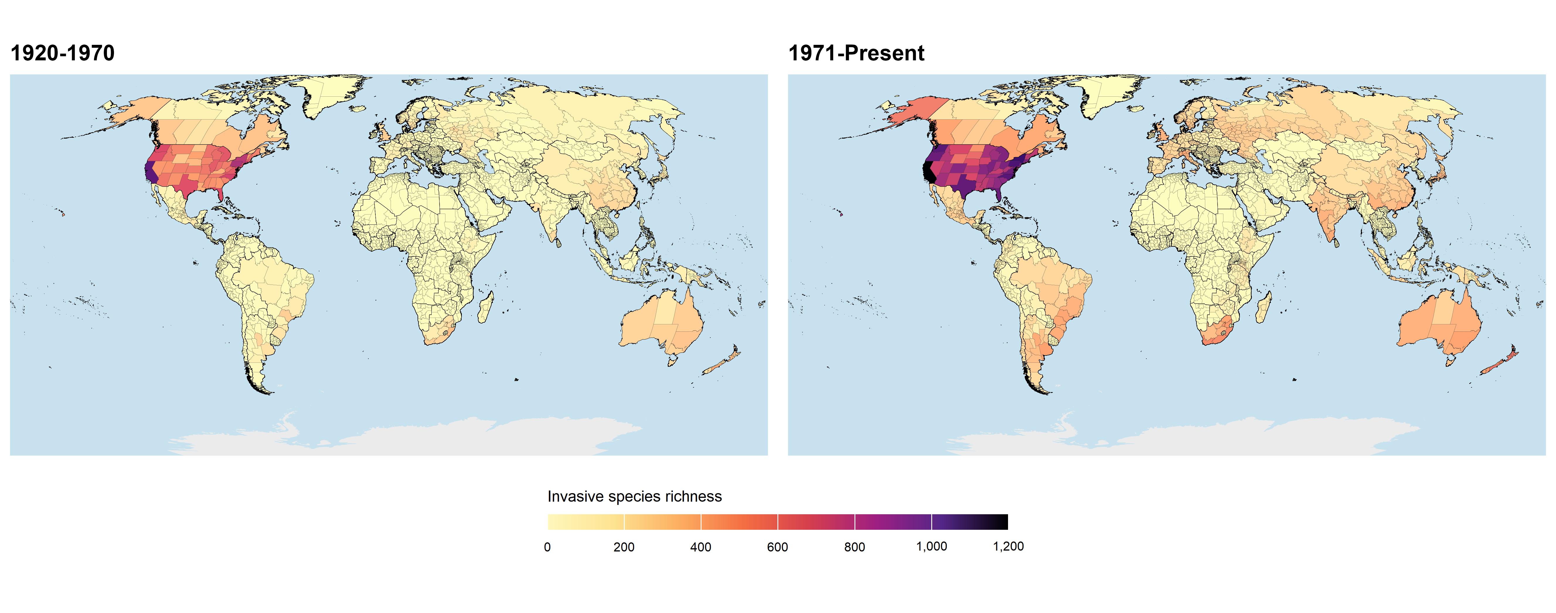
The terrestrial workflow focuses on assigning cleaned GBIF records to land-based spatial units. Users can summarise records by administrative boundaries, terrestrial ecoregions, protected areas and other landscape-context layers, depending on the spatial question being asked.

The example above shows invasive species richness summarised across subnational administrative units. In this case, biofetchR provides the cleaned and spatially attributed occurrence table; the map is then produced separately from that output.

Typical terrestrial use cases include:

assigning occurrence records to GADM administrative units;
summarising records by country, region or subnational unit;
comparing records with terrestrial ecoregions or protected-area layers;
preparing cleaned terrestrial occurrence tables for macroecological, conservation or invasion-biology analyses.

Freshwater occurrence workflows

Freshwater workflows focus on occurrence records whose ecological context is best described by inland-water systems, including rivers, lakes, reservoirs, wetlands, catchments and freshwater ecoregions. In biofetchR, occurrence records can be attributed to freshwater ecoregions, basins, river and lake layers, reservoirs, wetlands, Ramsar sites and related hydrological overlays.

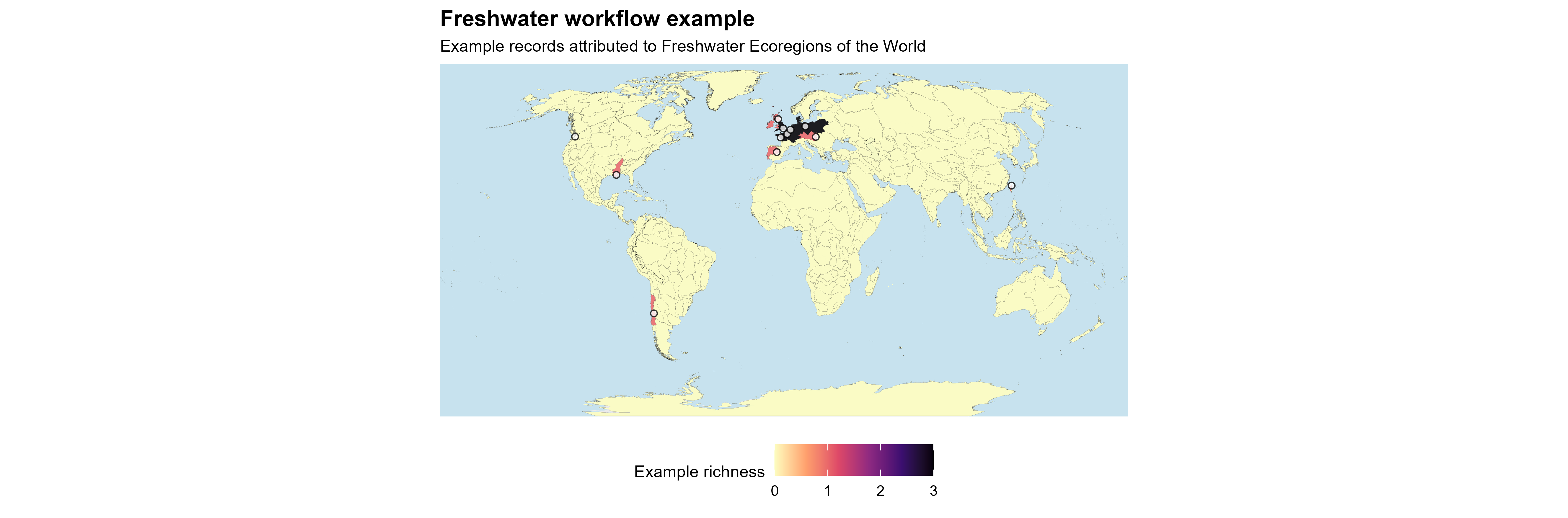
The example above summarises occurrence records against Freshwater Ecoregions of the World (FEOW). This is useful when the main question concerns drainage systems, freshwater biogeographic units, catchments or inland-water habitats, rather than broader terrestrial landscape contexts.

Typical freshwater use cases include:

assigning records to Freshwater Ecoregions of the World (FEOW);
summarising occurrences across basins, rivers, lakes or reservoirs;
linking records to wetland and Ramsar-site contexts;
identifying records that require freshwater-specific spatial interpretation;
preparing freshwater occurrence tables for analyses of species distributions, biological invasions, conservation priorities or invasion impacts.

Marine occurrence workflows

Marine workflows are designed to retain and interpret coastal, island and offshore records that may be excluded, misclassified or poorly summarised by land-focused occurrence workflows. In biofetchR, these records can be assigned to supported marine layers including EEZ-style units, Marine Regions products, IHO sea areas, Marine Ecoregions of the World and Large Marine Ecosystem (LME) polygons.

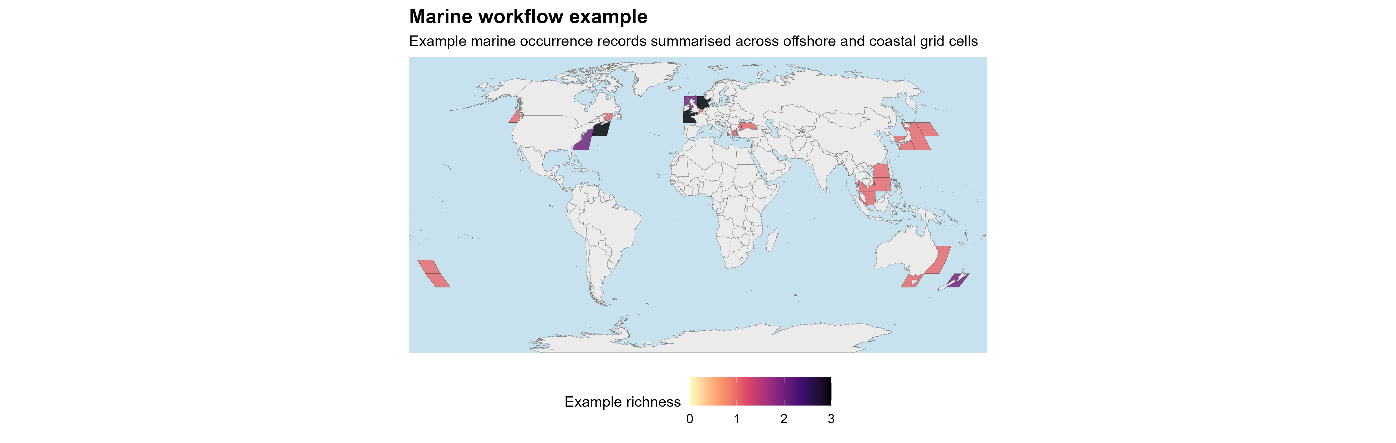
The example above shows marine records summarised across offshore and coastal grid cells. This provides a simple visual summary of where records occur, while the same workflow can also be used with named marine overlays when the question concerns jurisdictions, ecoregions, seas, shelves, islands, ports or other coastal and ocean contexts.

Typical marine use cases include:

retaining valid offshore records during occurrence processing;
assigning records to EEZ-style units or other marine jurisdictional layers;
summarising records by marine ecoregion, Large Marine Ecosystem or named sea area;
distinguishing coastal, island and open-water records from terrestrial spatial attribution;
preparing marine occurrence tables for biodiversity, biogeographic or biological-invasion analyses.

What biofetchR does

biofetchR is built around input tables that define the taxa and places to be processed, usually with one row per species-country combination and columns such as species and iso2c. For each row, the package can request matching GBIF occurrence records, import the completed download, clean and standardise the records, attach spatial context, add native-range or invasion-status evidence, and write processed outputs with diagnostic summaries.

Core workflow steps include:

reading an input table of species-country combinations, usually with species and iso2c columns;
resolving taxonomic names and GBIF taxon keys before downloads are submitted;
requesting and importing GBIF occurrence records for each input row;
standardising the returned records into consistent output tables;
applying coordinate-cleaning and optional spatial-thinning steps;
assigning records to the selected terrestrial, freshwater or marine workflow;
adding origin and invasion-status evidence where supported by the selected settings;
writing processed records, summaries and diagnostic files that document what happened during the run;
optionally saving separate output files for individual species-country combinations when large datasets need to be split into smaller files.

biofetchR keeps the main processing decisions visible. During a run, users can inspect how many records were returned, which records were removed during cleaning, where spatial joins succeeded or failed, and which evidence sources were used when assigning native, introduced or invasive status.

The resulting outputs are designed to be checked before analysis, rather than accepted as a single final table. This makes them suitable for biodiversity, macroecological, conservation and invasion-biology projects where occurrence records need to be cleaned, spatially attributed and interpreted consistently across many taxa or regions.

Installation

Install biofetchR outside package checks, following the installation instructions provided with the source repository.

Then load the package:

library(biofetchR)

Workflow summary

Most biofetchR workflows start from an input table of species-country combinations, usually with species and iso2c columns. Each row is treated as a processing unit: the package resolves the taxon, requests or reads the matching GBIF records for that country, applies the selected cleaning and spatial steps, and writes outputs to the chosen folder.

Workflow	Use when	Main output
Terrestrial	Records need to be interpreted using land-based boundaries or landscape-context layers	Cleaned occurrence records joined to the selected terrestrial overlays
Freshwater	Records are associated with inland-water systems or freshwater biogeographic units	Cleaned occurrence records joined to the selected freshwater overlays
Marine	Records are coastal, island-associated or offshore	Cleaned occurrence records joined to the selected marine overlays
Origin and status evidence	A workflow needs native-range, introduced-status or invasive-status information	Evidence fields that help interpret species-country origin and invasion status
Export options	Results need to be inspected, reused or split across a large batch	Combined outputs, diagnostic summaries and optional per-species-country files

These workflow components can be used separately or combined. For example, a species-country table can be processed through the terrestrial workflow, enriched with origin and status evidence, and exported either as one combined table or as separate files for each species-country combination.

The choice of workflow depends on the study system and the spatial question. A terrestrial analysis may require administrative units, a freshwater analysis may require hydrological context, and a marine analysis may require offshore or jurisdictional marine layers. The sections below show these options in more detail.

Terrestrial and freshwater workflows

Terrestrial and freshwater workflows usually start from a species-country input table. The simplest format is one row per species-country combination, with a species column and an ISO2 country code in iso2c.

terrestrial_input <- data.frame(
  species = c(
    "Xenopus laevis",
    "Trachemys scripta"
  ),
  iso2c = c(
    "FR",
    "GB"
  ),
  stringsAsFactors = FALSE
)

terrestrial_input
#>             species iso2c
#> 1    Xenopus laevis    FR
#> 2 Trachemys scripta    GB

The terrestrial example below requests GBIF records for each species-country combination, applies the selected cleaning and thinning settings, and assigns retained records to GADM level-1 administrative units.

result <- process_gbif_terrestrial_freshwater_pipeline(
  # Input table with one row per species-country combination.
  df = terrestrial_input,

  # Folder where processed records, summaries and diagnostics will be written.
  output_dir = file.path(example_output_root, "terrestrial_gadm"),

  # GBIF credentials. These are best stored as environment variables.
  user = Sys.getenv("GBIF_USER"),
  pwd = Sys.getenv("GBIF_PWD"),
  email = Sys.getenv("GBIF_EMAIL"),

  # Spatial overlay settings. Here, records are joined to GADM level-1 units.
  region_source = "gadm",
  gadm_unit = 1,

  # Record-cleaning settings.
  apply_cleaning = TRUE,
  apply_thinning = TRUE,
  dist_km = 5,

  # Output settings. For larger batches, write results to disk instead of
  # keeping all records in memory.
  export_summary = TRUE,
  store_in_memory = FALSE,
  return_all_results = FALSE
)

For freshwater analyses, the same input table can be processed with a freshwater-specific region_source. In this example, records are assigned to Freshwater Ecoregions of the World (FEOW).

freshwater_result <- process_gbif_terrestrial_freshwater_pipeline(
  df = terrestrial_input,

  output_dir = file.path(example_output_root, "freshwater_feow"),

  user = Sys.getenv("GBIF_USER"),
  pwd = Sys.getenv("GBIF_PWD"),
  email = Sys.getenv("GBIF_EMAIL"),

  # Use a freshwater overlay instead of an administrative boundary.
  region_source = "feow",

  apply_cleaning = TRUE,
  apply_thinning = TRUE,
  dist_km = 5,

  export_summary = TRUE,
  store_in_memory = FALSE,
  return_all_results = FALSE
)

freshwater_result <- process_gbif_terrestrial_freshwater_pipeline(
  df = terrestrial_input,

  output_dir = file.path(example_output_root, "freshwater_feow"),

  user = Sys.getenv("GBIF_USER"),
  pwd = Sys.getenv("GBIF_PWD"),
  email = Sys.getenv("GBIF_EMAIL"),

  # Use a freshwater overlay instead of an administrative boundary.
  region_source = "feow",

  apply_cleaning = TRUE,
  apply_thinning = TRUE,
  dist_km = 5,

  export_summary = TRUE,
  store_in_memory = FALSE,
  return_all_results = FALSE
)

For larger batches, store_in_memory = FALSE writes results to the output folder instead of holding them as one large R object. This is useful when users want outputs saved separately for individual species-country combinations.

Marine workflows

Marine workflows use a separate pipeline for coastal, offshore and other marine occurrence records. Unlike the terrestrial and freshwater examples above, the marine input can be a species table without a country column.

marine_input <- data.frame(
  species = c(
    "Carcinus maenas",
    "Undaria pinnatifida"
  ),
  stringsAsFactors = FALSE
)

marine_input
#>               species
#> 1     Carcinus maenas
#> 2 Undaria pinnatifida

The example below assigns marine occurrence records to EEZ-style polygons. Other supported marine overlays can be selected by changing the overlay argument.

marine_result <- process_gbif_marine_pipeline(
  df = marine_input,

  output_dir = file.path(example_output_root, "marine_eez"),

  user = Sys.getenv("GBIF_USER"),
  pwd = Sys.getenv("GBIF_PWD"),
  email = Sys.getenv("GBIF_EMAIL"),

  # Choose the marine overlay used for spatial attribution.
  overlay = "eez",
  overlay_cache_dir = file.path(example_cache_root, "marine_overlays"),

  apply_cleaning = TRUE,
  apply_thinning = TRUE,
  dist_km = 5,

  export_summary = TRUE,
  store_in_memory = FALSE,
  return_all_results = FALSE
)

Choose the marine overlay according to the spatial question. EEZ-style layers are useful for jurisdictional marine areas, Large Marine Ecosystem (LME) polygons for broad ecosystem regions, MEOW for coastal marine biogeography, and IHO sea areas for named seas or hydrographic regions.

Origin and invasive-status evidence

biofetchR can add origin and invasive-status fields to processed occurrence outputs before users decide whether to filter records. This separates occurrence processing from biological interpretation: a record can be cleaned and spatially attributed first, then assessed using the available evidence for whether the species is native, introduced, invasive or unresolved in that location.

The evidence sources used depend on the workflow and settings selected. GBIF, WoRMS and SInAS can contribute native-range or origin information, while GRIIS-style species-country records can support introduced or invasive-status classification. Because these sources differ in coverage, terminology and spatial resolution, biofetchR treats them as evidence fields that can be inspected rather than as a single automatic decision.

origin_result <- process_gbif_terrestrial_freshwater_pipeline(
  df = terrestrial_input,

  output_dir = file.path(example_output_root, "terrestrial_origin_audit"),

  user = Sys.getenv("GBIF_USER"),
  pwd = Sys.getenv("GBIF_PWD"),
  email = Sys.getenv("GBIF_EMAIL"),

  region_source = "gadm",
  gadm_unit = 1,

  # Add GRIIS-style introduced or invasive-status evidence, but do not
  # restrict the first run to invasive-only records.
  use_griis = TRUE,
  filter_griis_invasive = FALSE,

  # Add native-range evidence and export it for inspection.
  use_native_range = TRUE,
  use_native_web = TRUE,
  native_web_sources = c("sinas", "gbif"),
  native_filter_mode = "audit_only",

  # Combine available origin/status fields into a clearer audit output.
  reconcile_origin_evidence = TRUE,
  export_origin_audit = TRUE,

  apply_cleaning = TRUE,
  apply_thinning = TRUE,
  dist_km = 5,

  export_summary = TRUE,
  store_in_memory = FALSE,
  return_all_results = FALSE
)

In this example, the first run is evidence-based rather than filter-first. GRIIS-style information is attached, native-range evidence is queried, and the combined origin/status fields are exported for review. This lets users check which species-country combinations have consistent, conflicting or unresolved evidence before applying stricter filtering rules.

Typical origin and status use cases include:

checking whether records occur inside or outside available native-range evidence;
comparing origin/status fields from different sources;
identifying species-country combinations with uncertain or conflicting classifications;
exporting an origin-evidence table before removing records;
deciding whether an analysis should retain all records, introduced records, invasive records or a more conservative subset.

For publication-facing workflows, users should report which evidence sources were used, whether they were used for inspection or filtering, and how uncertain or conflicting classifications were handled.

Outputs and diagnostics

Most high-level biofetchR workflows write a gbif_summary.csv file to the selected output_dir. This file gives a row-by-row overview of the run, including which species-country combinations succeeded, which failed or returned no records, how many records were retained after processing, and where the exported files were saved.

The summary file is the best place to start after a batch run. It helps users spot failed downloads, missing output files, unexpectedly low record retention, or large differences between raw, cleaned and thinned record counts without opening every occurrence table individually.

Common gbif_summary.csv fields include:

Field	Meaning
`species`	Species name processed by the workflow
`status`	Whether the row succeeded, failed, returned no records or was skipped
`fail_stage`	Processing step where a failure occurred, where relevant
`fail_reason`	Short explanation of the failure or issue
`n_total`	Number of records returned before cleaning
`n_cleaned`	Number of records retained after coordinate cleaning
`n_thinned`	Number of records retained after optional spatial thinning
`output_file`	Path to the exported occurrence file for that row
`download_key`	GBIF download key, where available
`doi`	GBIF download DOI, where available
`region_source`	Spatial overlay used for attribution
`gadm_unit`	GADM administrative level, where relevant
`notes`	Additional processing notes, where generated

For larger analyses, useful files to keep include the original input table, gbif_summary.csv, exported occurrence files, origin-evidence outputs, spatial-attribution diagnostics, failed-row logs, GBIF download keys or DOIs, overlay-source metadata and sessionInfo() output.

A simple output folder might look like this:

outputs/
├── gbif_summary.csv
├── occurrence_files/
│   ├── Xenopus_laevis_FR.csv
│   └── Trachemys_scripta_GB.csv
├── audits/
│   ├── origin_evidence_audit.csv
│   ├── spatial_attribution_audit.csv
│   └── failed_rows.csv
├── cache/
│   ├── gbif/
│   └── spatial_overlays/
└── sessionInfo.txt

These files make the processing history easier to check and reuse. They show which input rows were processed, which records were retained or removed, which spatial layers were applied, and which origin or invasive-status evidence was attached. For publication-facing analyses, they should be kept with the main analysis outputs rather than treated as temporary files.

Recommended user guides

The package includes user guides for the main biofetchR workflows. These are best used as worked examples: they show how to structure inputs, choose settings, run pipelines and inspect the files written to the output folder.

Guide	File	Start here when you want to…
Batch pipelines	`biofetchR-batch-pipelines.Rmd`	run terrestrial or freshwater GBIF workflows for species-country tables
Origin evidence	`biofetchR-origin-evidence.Rmd`	add native-range, introduced-status or invasive-status evidence
Spatial overlays	`biofetchR-spatial-overlays.Rmd`	join cleaned records to administrative, ecological or contextual layers
Marine workflows	`biofetchR-marine-workflows.Rmd`	process coastal and offshore records with marine-region overlays
Auditing and scaling	`biofetchR-auditing-and-scaling.Rmd`	inspect outputs, diagnose failed rows and manage larger batches

New users should usually begin with the batch-pipelines guide, because it introduces the standard species-country input format and the main terrestrial and freshwater pipeline. The origin-evidence and spatial-overlays guides can then be used when a workflow needs biological status fields or additional spatial context. The marine guide covers the separate marine pipeline, and the auditing-and-scaling guide is useful before running larger input tables.

After installing biofetchR, all guides can be opened from R with:

browseVignettes("biofetchR")

Individual guides can also be opened directly:

vignette("biofetchR-batch-pipelines", package = "biofetchR")
vignette("biofetchR-origin-evidence", package = "biofetchR")
vignette("biofetchR-spatial-overlays", package = "biofetchR")
vignette("biofetchR-marine-workflows", package = "biofetchR")
vignette("biofetchR-auditing-and-scaling", package = "biofetchR")

Function-level help is available through the usual R help system:

?process_gbif_terrestrial_freshwater_pipeline
?process_gbif_marine_pipeline

Optional workflow dependencies

Most packages needed for standard biofetchR workflows are installed with the package. A smaller number of packages are only needed for particular features, such as raster-based overlays, geometry repair, OpenStreetMap layers, Natural Earth helpers or WoRMS queries.

These packages are treated as optional because not every user will need every provider or spatial-data source. For example, a basic GBIF occurrence workflow does not necessarily require packages used for raster layers, marine-origin lookups or OpenStreetMap-derived context.

If a selected workflow needs an optional package that is not installed, biofetchR will report the missing package. Install it, then rerun the workflow.

biofetchR::install_optional_deps()
#>               package                                         purpose available
#> 1           geosphere     Distance calculations and spatial utilities      TRUE
#> 2             ggplot2          Plotting examples and visual summaries      TRUE
#> 3                httr        HTTP requests for optional web workflows      TRUE
#> 4              lwgeom Geometry repair and advanced spatial operations      TRUE
#> 5  mapme.biodiversity            Optional biodiversity context layers      TRUE
#> 6             osmdata         OpenStreetMap-based contextual overlays      TRUE
#> 7              readxl                      Reading spreadsheet inputs      TRUE
#> 8       rnaturalearth               Natural Earth contextual overlays      TRUE
#> 9             stringi                       String encoding utilities      TRUE
#> 10            stringr                   String manipulation utilities      TRUE
#> 11              terra                        Raster context workflows      TRUE
#> 12              tidyr                        Data reshaping utilities      TRUE
#> 13             worrms      World Register of Marine Species workflows      TRUE

Common optional packages include:

Package	Used for
`terra`	Raster-based layers and selected spatial-data operations
`lwgeom`	Geometry repair and additional `sf` geometry operations
`osmdata`	OpenStreetMap-derived contextual layers
`rnaturalearth`	Natural Earth country, land and boundary layers
`worrms`	WoRMS taxonomic or marine-origin lookups

Some external spatial resources are large, provider-dependent or updated outside the package. These files may be downloaded during a workflow, stored in a local cache, or supplied by the user when a provider source is unavailable.

For larger or repeatable analyses, it is useful to define cache folders explicitly. This avoids repeated downloads and makes it easier to reuse the same overlay files across runs.

dir.create(example_cache_root, recursive = TRUE, showWarnings = FALSE)
dir.create(file.path(example_cache_root, "spatial_overlays"), recursive = TRUE, showWarnings = FALSE)
dir.create(file.path(example_cache_root, "marine_overlays"), recursive = TRUE, showWarnings = FALSE)
dir.create(file.path(example_cache_root, "native_range"), recursive = TRUE, showWarnings = FALSE)

Users should also keep a record of the package versions and external resources used in an analysis. At minimum, save sessionInfo() with the output folder and keep any overlay metadata or provider notes alongside the processed occurrence files.

writeLines(
  capture.output(sessionInfo()),
  file.path(example_output_root, "sessionInfo.txt")
)

Reproducibility

Reproducibility is central to biofetchR workflows. Occurrence datasets can change through time, spatial products can be updated, and cleaning or filtering settings can strongly affect the final records retained for analysis. For this reason, users should treat the exported occurrence tables and audit files as part of the analysis record, not as temporary intermediate files.

For publication-facing analyses, users should report:

GBIF download DOI or download key;
date of occurrence download or data access;
input species list and country or region fields used;
spatial overlay source, product name, version and access date;
coordinate-cleaning settings;
spatial-thinning settings and thinning distance, if thinning was used;
terrestrial, freshwater or marine spatial unit used for attribution;
origin-evidence sources and whether they were used for audit or filtering;
native-range or invasive-status filtering settings, if applied;
package version;
R version and session information.

A minimal reproducibility record can be saved with:

writeLines(
  capture.output(sessionInfo()),
  file.path(example_output_root, "sessionInfo.txt")
)

For larger analyses, users should also keep a copy of the exact input table and the main workflow summary file:

dir.create(file.path(example_output_root, "reproducibility"), recursive = TRUE, showWarnings = FALSE)

file.copy(
  from = "input_species_list.csv",
  to = "outputs/reproducibility/input_species_list.csv",
  overwrite = TRUE
)

file.copy(
  from = "outputs/gbif_summary.csv",
  to = "outputs/reproducibility/gbif_summary.csv",
  overwrite = TRUE
)

When external spatial overlays are used, the source and version should be recorded alongside the output files. This is important because administrative boundaries, protected-area layers, freshwater datasets and marine-region products may be revised over time.

overlay_metadata <- data.frame(
  overlay_name = c("GADM", "FEOW", "Marine Regions"),
  product = c("Administrative boundaries", "Freshwater ecoregions", "Marine overlay"),
  version = c("record_version_here", "record_version_here", "record_version_here"),
  access_date = as.character(Sys.Date()),
  source_url = c("record_url_here", "record_url_here", "record_url_here"),
  stringsAsFactors = FALSE
)

write.csv(
  overlay_metadata,
  file = "outputs/reproducibility/spatial_overlay_metadata.csv",
  row.names = FALSE
)

The aim is that another user, or the same user later, can reconstruct which records were downloaded, which records were removed, which spatial units were used, which evidence sources were applied, and which settings produced the final analysis-ready dataset.

Reproducibility

biofetchR outputs are designed to be kept with the analysis they support. A completed GBIF download can be linked back to its download key and DOI where available, while the package version and selected workflow settings show how the downloaded records were cleaned, filtered, spatially attributed and interpreted.

Rerunning the same species-country query later may create a new GBIF download if the workflow is submitted again. For this reason, users should keep the download key or DOI from the original run rather than relying only on the query that generated it.

For spatial attribution, users should record the workflow type and overlay used. For package-managed overlays, the biofetchR version is usually the most important reference point. If external, cached or user-supplied spatial files are used, any available source, version and access-date metadata should also be kept with the outputs.

For publication-facing analyses, useful details to report include:

Item	What to record
Input data	Input table, species names and country or region fields used
GBIF data	Download key, DOI where available and download or access date
Cleaning	Coordinate-cleaning settings and record filters applied
Thinning	Whether thinning was used and the thinning distance
Spatial attribution	Workflow type, selected overlay and relevant overlay settings
Origin/status evidence	Evidence sources used and whether they were used for audit or filtering
External resources	Source, version or access-date metadata for cached or user-supplied files
Software	`biofetchR` version, R version and package session information

A minimal reproducibility folder can be created inside the output directory:

dir.create(file.path(example_output_root, "reproducibility"), recursive = TRUE, showWarnings = FALSE)

writeLines(
  capture.output(sessionInfo()),
  file.path(example_output_root, "reproducibility", "sessionInfo.txt")
)

Users should also keep the original input table and the main workflow summary. Together, these files show what was submitted to the workflow and what happened to each input row.

file.copy(
  from = "input_species_list.csv",
  to = file.path(example_output_root, "reproducibility", "input_species_list.csv"),
  overwrite = TRUE
)

file.copy(
  from = file.path(example_output_root, "gbif_summary.csv"),
  to = file.path(example_output_root, "reproducibility", "gbif_summary.csv"),
  overwrite = TRUE
)

When external or user-supplied overlays are used, a small metadata table can be saved alongside the processed occurrence files.

overlay_metadata <- data.frame(
  overlay_name = c("custom_overlay_name"),
  source = c("record_source_here"),
  version = c("record_version_here"),
  access_date = as.character(Sys.Date()),
  notes = c("record_any_relevant_processing_or_cache_notes_here"),
  stringsAsFactors = FALSE
)

write.csv(
  overlay_metadata,
  file = file.path(
    "outputs",
    "reproducibility",
    "external_overlay_metadata.csv"
  ),
  row.names = FALSE
)

These records make it easier to rerun the workflow, explain why records were retained or removed, identify which spatial settings were used, and describe how native-range or invasive-status evidence was handled.

README figures

The figures in this README are static PNG files stored in man/figures/:

man/figures/readme-terrestrial-richness.png
man/figures/readme-freshwater-feow.png
man/figures/readme-marine-regions.png

They are included to show examples of the spatial summaries that can be produced after running biofetchR workflows. The package itself does not provide plotting functions. Instead, it writes processed occurrence tables that users can map with standard R tools such as sf, ggplot2, terra or other spatial-visualisation packages.

Using static images keeps the README fast to render and easy to view on GitHub. It also avoids rerunning GBIF downloads, loading large spatial overlays or querying external providers each time the README is built.

The figure files can be regenerated during package development using scripts in:

dev/readme_figures/

These scripts are separate from the exported package functions. They are used only to prepare the README images and may depend on local example data, cached spatial layers or other development files.

To update the README figures, regenerate or replace the PNG files in man/figures/, then rerender the README:

rmarkdown::render("README.Rmd")

If the README is rendered before the PNG files are available, the figure panels should be checked carefully before committing the updated README. The static image files should be committed with the README so that users can view the figures without running the development scripts.

Citation

When using biofetchR, cite the package and the data sources that contributed to the final dataset. biofetchR should be cited for the workflow used to download, clean, classify, enrich and export occurrence records, while external providers should be cited for the occurrence, taxonomic, spatial or status evidence used in the analysis.

For the package itself, cite the version, release or repository commit used in the analysis. Where available, the package citation can be checked from R:

citation("biofetchR")

GBIF-mediated occurrence records should be cited using the GBIF download DOI created for the download used in the analysis. The DOI identifies the downloaded dataset and gives credit to the underlying data publishers. Users do not need to cite each individual occurrence record separately. If a DOI is not available, retain and report the GBIF download key.

Cite external providers only when they were actually used in the workflow. For example, a terrestrial workflow may require a GBIF download DOI and a citation for the boundary layer used for spatial attribution. A marine workflow may also require citation of Marine Regions, WoRMS or another marine data provider. A workflow using native-range or invasive-status evidence should cite the relevant evidence source separately.

Useful citation details include:

Resource	What to cite
`biofetchR`	Package version, release or repository commit
GBIF occurrence records	GBIF download DOI, or download key if a DOI is unavailable
Spatial overlays	Product name, provider, version and access date where relevant
Taxonomic services	Source used for taxonomic matching or validation
Origin/status evidence	Native-range, introduced-status or invasive-status evidence source
Custom data	Any user-supplied occurrence tables or spatial layers used in the workflow

A publication-facing citation record might include:

biofetchR package version or repository commit
GBIF download DOI for occurrence records
Spatial overlay product used for attribution
Taxonomic or marine-origin provider, where applicable
Native-range or invasive-status evidence source, where applicable

Users should avoid citing only biofetchR when the analysis also depends on external occurrence records, spatial products or evidence sources. The clearest approach is to cite biofetchR for the processing workflow and cite each underlying provider for the data used to build the final dataset.

Package status

biofetchR is a developing research software package for biodiversity occurrence-data workflows. The core terrestrial, freshwater, marine, origin evidence and export workflows are being refined through continued testing across additional taxa, regions and spatial data sources.

Future updates may expand spatial-overlay support, improve diagnostics, add new provider options and incorporate additional databases for assessing non-native or invasive status. These additions will build on the existing evidence-based approach, where external sources are used to support interpretation rather than being treated as a single definitive classification.

Users running larger analyses should record the package version or repository commit used, especially when results need to be reproduced later.

packageVersion("biofetchR")

Before rerunning an older analysis with a newer version of the package, users should check whether any relevant arguments, defaults, provider requirements, evidence sources or output formats have changed.

mirror server hosted at Truenetwork, Russian Federation.