
![]()


![]()
![]()
![]()
dfms provides efficient estimation of Dynamic Factor Models
in R via the EM Algorithm. Factors are assumed to follow a stationary
VAR process of order p. Estimation can be done in 3
different ways following:
Doz, C., Giannone, D., & Reichlin, L. (2011). A two-step estimator for large approximate dynamic factor models based on Kalman filtering. Journal of Econometrics, 164(1), 188-205. doi:10.1016/j.jeconom.2011.02.012
Doz, C., Giannone, D., & Reichlin, L. (2012). A quasi-maximum likelihood approach for large, approximate dynamic factor models. Review of Economics and Statistics, 94(4), 1014-1024. doi:10.1162/REST_a_00225
Banbura, M., & Modugno, M. (2014). Maximum likelihood estimation of factor models on datasets with arbitrary pattern of missing data. Journal of Applied Econometrics, 29(1), 133-160. doi:10.1002/jae.2306
The default is em.method = "auto", which chooses
"BM" following Banbura & Modugno (2014) with missing
data or mixed frequency, and "DGR" following Doz, Giannone
& Reichlin (2012) otherwise. Using em.method = "none"
generates Two-Step estimates following Doz, Giannone & Reichlin
(2011). This is extremely efficient on bigger datasets. PCA and Two-Step
estimates are also reported in EM-estimation. All methods support
missing data, but em.method = "DGR" does not model them in
EM iterations.
The package is now at a 1.0.0 release and includes
news() for Banbura and Modugno (2014) style news
decomposition of forecast updates.
dfms provides a simple, numerically robust, and
computationally efficient implementation of (linear Gaussian) Dynamic
Factor Models for R, allowing straightforward application to time series
dimensionality reduction, forecasting, and nowcasting tasks. It is based
on efficient C++ code, making dfms orders of magnitude faster
than other packages that can be used to fit dynamic factor models such
as MARSS, or
nowcasting
and nowcastDFM
geared to mixed-frequency nowcasting applications - which dfms
now also supports. For large-scale nowcasting models the DynamicFactorMQ
class in the statsmodels Python library is likely the best
implementation - see the example
by Chad Fulton.
The dfms package is not intended to fit more general forms of
the state space model like MARSS.
# CRAN
install.packages("dfms")

# Development Version
install.packages('dfms', repos = c('https://ropensci.r-universe.dev', 'https://cloud.r-project.org'))library(dfms)
# Fit DFM with 6 factors and 3 lags in the transition equation
mod <- DFM(diff(BM14_M), r = 6, p = 3) ## Converged after 32 iterations.# 'dfm' methods
summary(mod)## Dynamic Factor Model: n = 92, T = 356, r = 6, p = 3, %NA = 25.8366
##
## Call: DFM(X = diff(BM14_M), r = 6, p = 3)
##
## Summary Statistics of Factors [F]
## N Mean Median SD Min Max
## f1 356 -0.1189 0.4409 4.0228 -22.9164 7.8513
## f2 356 -0.4615 -0.3476 2.9201 -9.0973 10.7003
## f3 356 -0.0173 0.0377 2.2719 -8.5067 7.3009
## f4 356 -0.007 -0.1338 1.9378 -9.5052 9.3673
## f5 356 0.237 0.1091 2.0857 -8.7252 9.6715
## f6 356 -0.8361 -0.304 3.1406 -11.6611 15.4897
##
## Factor Transition Matrix [A]
## L1.f1 L1.f2 L1.f3 L1.f4 L1.f5 L1.f6 L2.f1 L2.f2 L2.f3
## f1 0.53029 -0.53009 0.367302 0.04607 -0.06351 0.10310 0.02457 0.11673 -0.12638
## f2 -0.28380 0.07421 -0.032292 0.29741 -0.10094 0.21989 0.09958 -0.09149 0.06708
## f3 0.17607 0.12979 0.378798 -0.06662 -0.12236 0.06685 -0.08068 0.09101 -0.22232
## f4 0.02711 0.08936 0.004643 0.37159 0.12100 -0.02763 0.01234 -0.05147 0.02195
## f5 -0.26227 -0.03469 -0.046294 0.12712 0.26847 0.03141 0.06400 0.01971 0.04806
## f6 0.08251 0.17619 -0.013374 -0.08731 -0.03875 0.27812 -0.01662 0.04877 0.02279
## L2.f4 L2.f5 L2.f6 L3.f1 L3.f2 L3.f3 L3.f4 L3.f5 L3.f6
## f1 0.23135 0.117184 0.21941 0.18478 0.02259 -0.03719 -0.07236 -0.03026 -0.12606
## f2 -0.09768 -0.043057 0.08489 0.21107 0.16261 0.03057 0.04835 0.12249 0.13357
## f3 0.09799 -0.060666 -0.18028 -0.02773 0.01798 0.10143 -0.12420 0.04207 -0.07011
## f4 0.01266 0.050912 0.05144 -0.05601 0.04665 0.05710 -0.11412 -0.05680 -0.01609
## f5 -0.03965 -0.009952 -0.18471 0.08332 -0.04640 -0.02047 0.02458 0.16397 0.07820
## f6 0.01163 -0.100859 0.07152 0.00792 0.06071 0.11381 0.02520 -0.17897 0.30328
##
## Factor Covariance Matrix [cov(F)]
## f1 f2 f3 f4 f5 f6
## f1 16.1832 -0.4329 0.2483 -0.8224* -1.7708* 0.7702
## f2 -0.4329 8.5272 0.0051 0.2954 -0.2114 4.2080*
## f3 0.2483 0.0051 5.1614 -0.1851 -0.3979 0.2979
## f4 -0.8224* 0.2954 -0.1851 3.7550 0.4344* 0.2211
## f5 -1.7708* -0.2114 -0.3979 0.4344* 4.3503 -1.9785*
## f6 0.7702 4.2080* 0.2979 0.2211 -1.9785* 9.8634
##
## Factor Transition Error Covariance Matrix [Q]
## u1 u2 u3 u4 u5 u6
## u1 7.2142 0.1151 -0.8208 -0.4379 0.4110 -0.1206
## u2 0.1151 4.8724 0.1076 -0.1438 0.1418 0.1759
## u3 -0.8208 0.1076 4.0584 -0.0788 0.0163 0.0038
## u4 -0.4379 -0.1438 -0.0788 3.0003 0.2562 0.0243
## u5 0.4110 0.1418 0.0163 0.2562 2.8410 -0.1031
## u6 -0.1206 0.1759 0.0038 0.0243 -0.1031 2.9284
##
## Summary of Residual AR(1) Serial Correlations
## N Mean Median SD Min Max
## 92 -0.0644 -0.1024 0.2702 -0.5113 0.6674
##
## Summary of Individual R-Squared's
## N Mean Median SD Min Max
## 92 0.4556 0.4069 0.3041 0.0112 0.9989plot(mod)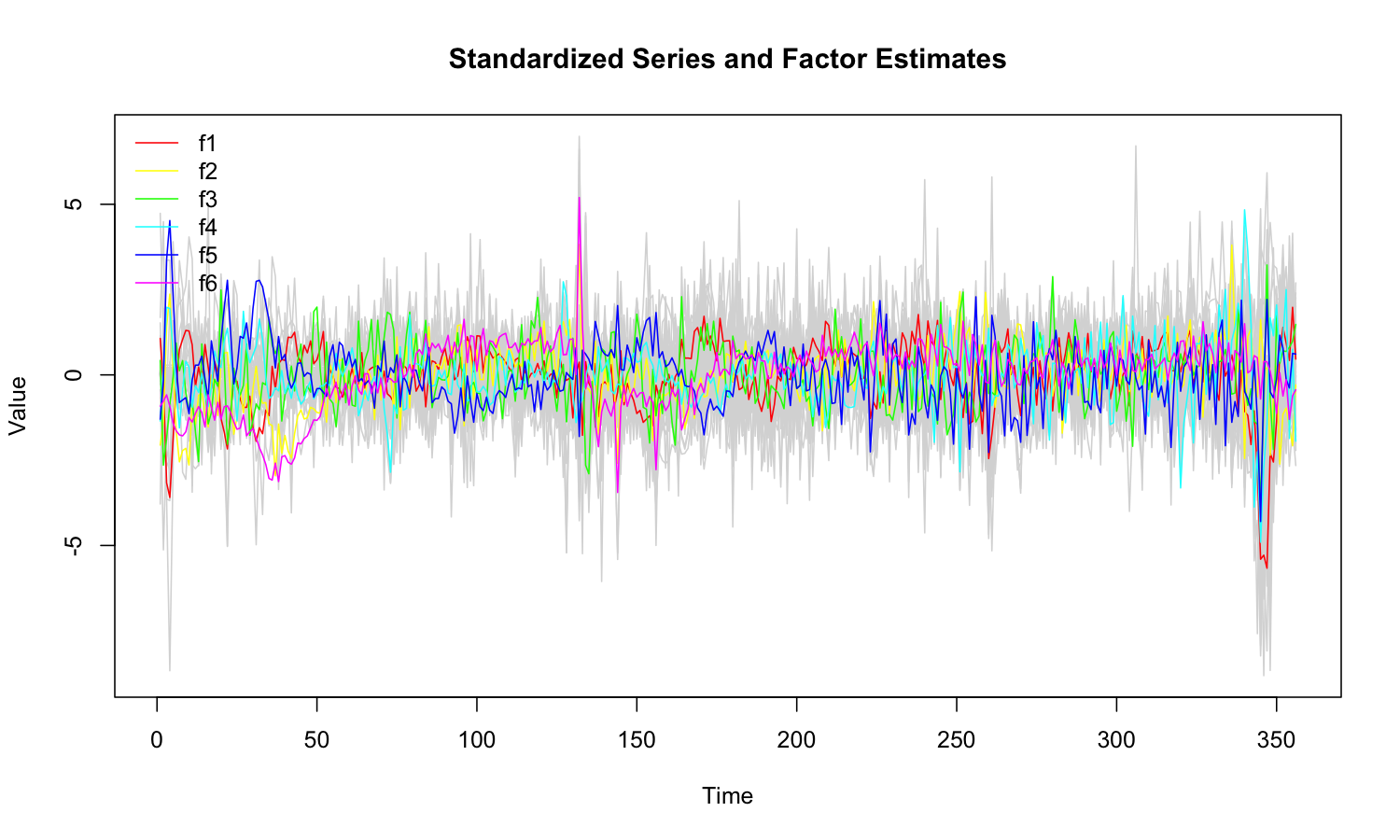
as.data.frame(mod) |> head()## Method Factor Time Value
## 1 PCA f1 1 0.8445713
## 2 PCA f1 2 0.5259228
## 3 PCA f1 3 -1.2107116
## 4 PCA f1 4 -1.5399532
## 5 PCA f1 5 -0.4631786
## 6 PCA f1 6 0.2399304# Forecasting 12 periods ahead
fc <- predict(mod, h = 12)
# 'dfm_forecast' methods
plot(fc, xlim = c(320, 370))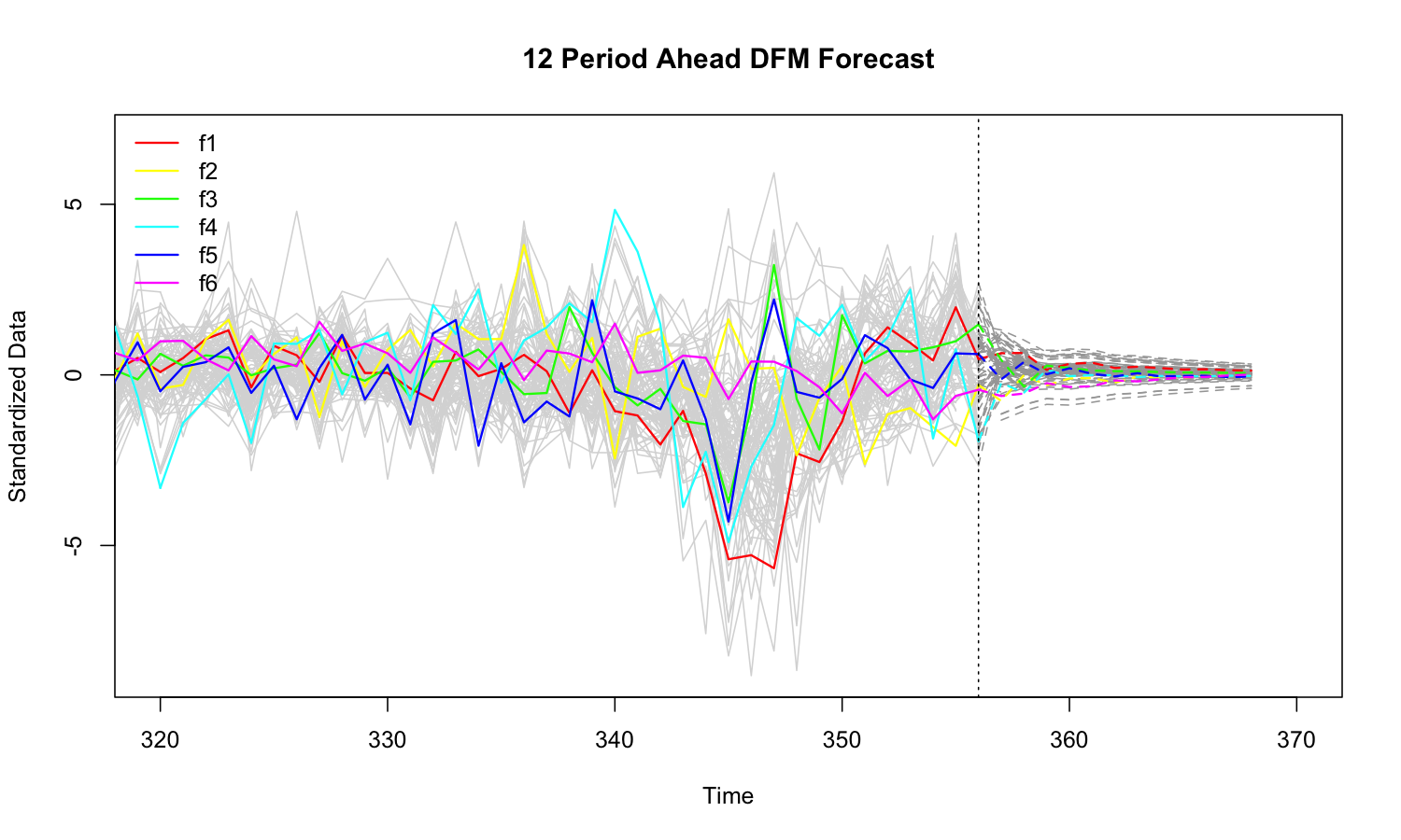
as.data.frame(fc) |> head()## Variable Time Forecast Value
## 1 f1 1 FALSE 4.179331
## 2 f1 2 FALSE -1.368577
## 3 f1 3 FALSE -12.845157
## 4 f1 4 FALSE -14.562265
## 5 f1 5 FALSE -7.791254
## 6 f1 6 FALSE -1.254970