



lbugr provides an R interface to the Ladybug Graph Database, a
high-performance, embedded graph database. The package acts as a wrapper
around the official Python ladybug client, using the
reticulate package to bridge the two languages. This allows
you to interact with Ladybug seamlessly within your R environment,
integrating its powerful graph computation capabilities into your
existing data analysis workflows.
The primary goal of lbugr is to provide an idiomatic R
experience for: - Creating and managing Ladybug database instances. -
Executing Cypher queries. - Loading data from and retrieving results
into R data frames and tibbles. - Converting graph query results
directly into R-native graph objects like igraph and
tidygraph.
lbugr requires Python 3.14 or later
with the ladybug package.
Note: Python 3.14+ is required due to fixes in the underlying kuzu database engine that resolve VirtualAlloc memory issues.
You can install the stable version from CRAN:
install.packages("lbugr")Or install the development version from GitHub:
# install.packages("pak")
pak::pak("WickM/lbugr")After installing lbugr, you must install the required
Python packages. You can do this from your R console using
reticulate:
library(lbugr)
reticulate::py_install("ladybug", pip = TRUE)Important: Ensure you have Python 3.14 or later installed. You can verify your Python version with
py -3.14 --version(Windows) orpython3 --version(macOS/Linux).
You can check that all dependencies are correctly installed by running:
check_ladybug_installation()
#> The 'ladybug' Python package is installed and available.Here is a complete example demonstrating how to create a database, define a schema, load data, and run queries.
library(lbugr)
library(igraph)
library(tidygraph)

# 1. Create a database in a temporary directory
db_path <- tempfile()
con <- lb_connection(db_path)

# 2. Define a schema
# Create a 'Person' node table with a STRING name and INT64 age
schema_query_1 <- "CREATE NODE TABLE Person (
  name STRING,
  age INT64,
  PRIMARY KEY (name)
)"
lb_execute(con, schema_query_1)
#>                           result
#> 1 Table Person has been created.

# Create a 'Knows' relationship table
schema_query_2 <- "CREATE REL TABLE Knows(FROM Person TO Person, since INT64)"
lb_execute(con, schema_query_2)
#>                          result
#> 1 Table Knows has been created.

# 3. Load data from R data frames
# Create node data
nodes <- data.frame(
  name = c("Alice", "Bob", "Carol"),
  age = c(30, 40, 50)
)

# Create edge data
edges <- data.frame(
  from_person = c("Alice", "Bob"),
  to_person = c("Bob", "Carol"),
  since = c(2010, 2015)
)

# Use lb_copy_from_df to load the data
lb_copy_from_df(con, nodes, "Person")

names(edges) <- c("FROM", "TO", "since")
lb_copy_from_df(con, edges, "Knows")

# 4. Execute Cypher queries
# Retrieve data as a data frame
query_result <- lb_execute(con, "MATCH (p:Person) RETURN p.name, p.age")
as.data.frame(query_result)
#>   p.name p.age
#> 1  Alice    30
#> 2    Bob    40
#> 3  Carol    50

# 5. Convert graph results to R objects
# The same query result can be converted into different graph formats.
graph_result <- lb_execute(con, "MATCH (a:Person)-[k:Knows]->(b:Person) RETURN a, k, b")

# a) Convert to an igraph object
g_igraph <- as_igraph(graph_result)
print(g_igraph)
#> IGRAPH 92733d3 DN-- 3 2 --
#> + attr: name (v/c), label (v/l), age (v/l)
#> + edges from 92733d3 (vertex names):
#> [1] Person:Alice->Person:Bob   Person:Bob  ->Person:Carol
plot(g_igraph,
     vertex.color = "#dc2626",
     vertex.label.color = "#f3f4f6",
     vertex.label.font = 2,
     edge.color = "#9ca3af",
     edge.arrow.size = 0.8,
     edge.arrow.width = 0.5,
     bg = "#030712",
     main = "lbugr Graph Structure")

# b) Convert to a tidygraph object
g_tidy <- as_tidygraph(graph_result)
print(g_tidy)
#> # A tbl_graph: 6 nodes and 2 edges
#> #
#> # A rooted forest with 4 trees
#> #
#> # Node Data: 6 × 3 (active)
#>   name         label    age
#>   <chr>        <chr>  <int>
#> 1 Person:Alice <NA>      NA
#> 2 Person:Bob   <NA>      NA
#> 3 Person:Carol <NA>      NA
#> 4 Alice        Person    30
#> 5 Bob          Person    40
#> 6 Carol        Person    50
#> #
#> # Edge Data: 2 × 2
#>    from    to
#>   <int> <int>
#> 1     1     2
#> 2     2     3

# 6. Inspecting Query Results
# You can inspect the schema of a query result without converting it to a data frame.
# Get column names
lb_get_column_names(query_result)
#> [1] "p.name" "p.age"

# Get column data types
lb_get_column_data_types(query_result)
#>      p.name       p.age
#> "character"   "integer"

# Get the full schema as a named list
lb_get_schema(query_result)
#>      p.name       p.age
#> "character"   "integer"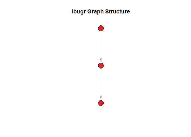
Plot of the graph structure created from Ladybug query results.