![]()
![]()
ledger is an R package to import data from plain text accounting
software like Ledger, HLedger, and Beancount into an R
data frame for convenient analysis, plotting, and export.
Right now it supports reading in the register from
ledger, hledger, and beancount
files.
To install the last version released to CRAN use the following command in R:
install.packages("ledger")To install the development version of the ledger package
(and its R package dependencies) use the install_github
function from the remotes package in R:
install.packages("remotes")
remotes::install_github("trevorld/r-ledger")
This package also has some system dependencies that need to be installed depending on which plaintext accounting files you wish to read:
To install hledger run the following in your shell:
stack update && stack install --resolver=lts-14.3 hledger-lib-1.15.2 hledger-1.15.2 hledger-web-1.15 hledger-ui-1.15 --verbosity=errorTo install bean-query (to read beancount
files) run the following in your shell:
pip3 install beanqueryAlternatively, install rledger from rustledger (>=
0.15.0).
Several pre-compiled Ledger binaries are available (often found in several open source repos).
The main function of this package is register() which
reads in the register of a plaintext accounting file. This package also
registers S3 methods so one can use rio::import() to read
in a register, a net_worth() convenience function, and a
prune_coa() convenience function.
register()Here are some examples of very basic files stored within the package:
library("ledger")
ledger_file <- system.file("extdata", "example.ledger", package = "ledger")
register(ledger_file)
## # A tibble: 42 × 9
## date mark payee description code account amount commodity comment
## <date> <chr> <chr> <chr> <chr> <chr> <dbl> <chr> <chr>
## 1 2015-12-31 * <NA> Opening Ba… <NA> Assets… 5000 USD ""
## 2 2015-12-31 * <NA> Opening Ba… <NA> Equity… -5000 USD ""
## 3 2016-01-01 * Landlord Rent <NA> Assets… -1500 USD ""
## 4 2016-01-01 * Landlord Rent <NA> Expens… 1500 USD ""
## 5 2016-01-01 * Brokerage Buy Stock <NA> Assets… -1000 USD ""
## 6 2016-01-01 * Brokerage Buy Stock <NA> Equity… 1000 USD ""
## 7 2016-01-01 * Brokerage Buy Stock <NA> Assets… 4 SP ""
## 8 2016-01-01 * Brokerage Buy Stock <NA> Equity… -1000 USD ""
## 9 2016-01-01 * Supermar… Grocery st… <NA> Expens… 501. USD "Link:…
## 10 2016-01-01 * Supermar… Grocery st… <NA> Liabil… -501. USD "Link:…
## # ℹ 32 more rowshledger_file <- system.file("extdata", "example.hledger", package = "ledger")
register(hledger_file)## # A tibble: 42 × 12
## date mark payee description account amount commodity historical_cost
## <date> <chr> <chr> <chr> <chr> <dbl> <chr> <dbl>
## 1 2015-12-31 * <NA> Opening Ba… Assets… 5000 USD 5000
## 2 2015-12-31 * <NA> Opening Ba… Equity… -5000 USD -5000
## 3 2016-01-01 * Landlo… Rent Assets… -1500 USD -1500
## 4 2016-01-01 * Landlo… Rent Expens… 1500 USD 1500
## 5 2016-01-01 * Broker… Buy Stock Assets… -1000 USD -1000
## 6 2016-01-01 * Broker… Buy Stock Equity… 1000 USD 1000
## 7 2016-01-01 * Broker… Buy Stock Assets… 4 SP 1000
## 8 2016-01-01 * Broker… Buy Stock Equity… -1000 USD -1000
## 9 2016-01-01 * Superm… Grocery st… Expens… 501. USD 501.
## 10 2016-01-01 * Superm… Grocery st… Liabil… -501. USD -501.
## # ℹ 32 more rows
## # ℹ 4 more variables: hc_commodity <chr>, market_value <dbl>,
## # mv_commodity <chr>, id <chr>beancount_file <- system.file("extdata", "example.beancount", package = "ledger")
register(beancount_file)## # A tibble: 42 × 13
## date mark payee description account amount commodity historical_cost
## <date> <chr> <chr> <chr> <chr> <dbl> <chr> <dbl>
## 1 2015-12-31 * "" Opening Ba… Assets… 5000 USD 5000
## 2 2015-12-31 * "" Opening Ba… Equity… -5000 USD -5000
## 3 2016-01-01 * "Landl… Rent Assets… -1500 USD -1500
## 4 2016-01-01 * "Landl… Rent Expens… 1500 USD 1500
## 5 2016-01-01 * "Broke… Buy Stock Assets… -1000 USD -1000
## 6 2016-01-01 * "Broke… Buy Stock Equity… 1000 USD 1000
## 7 2016-01-01 * "Broke… Buy Stock Assets… 4 SP 1000
## 8 2016-01-01 * "Broke… Buy Stock Equity… -1000 USD -1000
## 9 2016-01-01 * "Super… Grocery st… Expens… 501. USD 501.
## 10 2016-01-01 * "Super… Grocery st… Liabil… -501. USD -501.
## # ℹ 32 more rows
## # ℹ 5 more variables: hc_commodity <chr>, market_value <dbl>,
## # mv_commodity <chr>, tags <chr>, id <chr>Here is an example reading in a beancount file generated by
bean-example:
bean_example_file <- tempfile(fileext = ".beancount")
system(paste("bean-example -o", bean_example_file), ignore.stderr = TRUE)
df <- register(bean_example_file)
print(df)
## # A tibble: 2,898 × 13
## date mark payee description account amount commodity historical_cost
## <date> <chr> <chr> <chr> <chr> <dbl> <chr> <dbl>
## 1 2024-01-01 * "" Opening Ba… Assets… 3664. USD 3664.
## 2 2024-01-01 * "" Opening Ba… Equity… -3664. USD -3664.
## 3 2024-01-01 * "" Allowed co… Income… -18500 IRAUSD -18500
## 4 2024-01-01 * "" Allowed co… Assets… 18500 IRAUSD 18500
## 5 2024-01-03 * "Rive… Paying the… Assets… -2400 USD -2400
## 6 2024-01-03 * "Rive… Paying the… Expens… 2400 USD 2400
## 7 2024-01-04 * "BANK… Monthly ba… Assets… -4 USD -4
## 8 2024-01-04 * "BANK… Monthly ba… Expens… 4 USD 4
## 9 2024-01-04 * "Hool… Payroll Assets… 1351. USD 1351.
## 10 2024-01-04 * "Hool… Payroll Assets… 1200 USD 1200
## # ℹ 2,888 more rows
## # ℹ 5 more variables: hc_commodity <chr>, market_value <dbl>,
## # mv_commodity <chr>, tags <chr>, id <chr>suppressPackageStartupMessages(library("dplyr"))
dplyr::filter(df, grepl("Expenses", account), grepl("trip", tags)) %>%
group_by(trip = tags, account) %>%
summarize(trip_total = sum(amount), .groups = "drop")## # A tibble: 5 × 3
## trip account trip_total
## <chr> <chr> <dbl>
## 1 trip-chicago-2024 Expenses:Food:Alcohol 67.3
## 2 trip-chicago-2024 Expenses:Food:Coffee 48.4
## 3 trip-chicago-2024 Expenses:Food:Restaurant 483.
## 4 trip-san-francisco-2025 Expenses:Food:Coffee 24.4
## 5 trip-san-francisco-2025 Expenses:Food:Restaurant 745.rio::import()
and rio::convert()If one has loaded in the ledger package one can also use
rio::import() to read in the register:
df2 <- rio::import(bean_example_file)
all.equal(df, tibble::as_tibble(df2))
## [1] TRUEThe main advantage of this is that it allows one to use
rio::convert to easily convert plaintext accounting files
to several other file formats such as a csv file. Here is a shell
example:
bean-example -o example.beancount
Rscript --default-packages=ledger,rio -e 'convert("example.beancount", "example.csv")'net_worth()Some examples of using the net_worth function using the
example files from the register examples:
dates <- seq(as.Date("2016-01-01"), as.Date("2018-01-01"), by = "years")
net_worth(ledger_file, dates)
## # A tibble: 3 × 6
## date commodity net_worth assets liabilities revalued
## <date> <chr> <dbl> <dbl> <dbl> <dbl>
## 1 2016-01-01 USD 5000 5000 0 0
## 2 2017-01-01 USD 4361. 4882 -521. 0
## 3 2018-01-01 USD 6743. 6264 -521. 1000net_worth(hledger_file, dates)## # A tibble: 3 × 5
## date commodity net_worth assets liabilities
## <date> <chr> <dbl> <dbl> <dbl>
## 1 2016-01-01 USD 5000 5000 0
## 2 2017-01-01 USD 4361. 4882 -521.
## 3 2018-01-01 USD 6743. 7264 -521.net_worth(beancount_file, dates)## # A tibble: 3 × 5
## date commodity net_worth assets liabilities
## <date> <chr> <dbl> <dbl> <dbl>
## 1 2016-01-01 USD 5000 5000 0
## 2 2017-01-01 USD 4361. 4882 -521.
## 3 2018-01-01 USD 6743. 7264 -521.dates <- seq(min(as.Date(df$date)), max(as.Date(df$date)), by = "years")
net_worth(bean_example_file, dates)## # A tibble: 6 × 5
## date commodity net_worth assets liabilities
## <date> <chr> <dbl> <dbl> <dbl>
## 1 2025-01-01 IRAUSD 0 0 0
## 2 2025-01-01 USD 41983. 42888. -905.
## 3 2025-01-01 VACHR 10 10 0
## 4 2026-01-01 IRAUSD 0 0 0
## 5 2026-01-01 USD 79081. 80733. -1652.
## 6 2026-01-01 VACHR 20 20 0prune_coa()Some examples using the prune_coa function to simplify
the “Chart of Account” names to a given maximum depth:
suppressPackageStartupMessages(library("dplyr"))
df <- register(bean_example_file) %>% dplyr::filter(!is.na(commodity))
df %>%
    prune_coa() %>%
    group_by(account, mv_commodity) %>%
    summarize(market_value = sum(market_value), .groups = "drop")
## # A tibble: 11 × 3
## account mv_commodity market_value
## <chr> <chr> <dbl>
## 1 Assets IRAUSD 4100
## 2 Assets USD 104595.
## 3 Assets VACHR 80
## 4 Equity USD -3664.
## 5 Expenses IRAUSD 51400
## 6 Expenses USD 230242.
## 7 Expenses VACHR 240
## 8 Income IRAUSD -55500
## 9 Income USD -324422.
## 10 Income VACHR -320
## 11 Liabilities USD -2127.df %>%
prune_coa(2) %>%
group_by(account, mv_commodity) %>%
summarize(market_value = sum(market_value), .groups = "drop")## # A tibble: 17 × 3
## account mv_commodity market_value
## <chr> <chr> <dbl>
## 1 Assets:US IRAUSD 4.1 e+ 3
## 2 Assets:US USD 1.05e+ 5
## 3 Assets:US VACHR 8 e+ 1
## 4 Equity:Opening-Balances USD -3.66e+ 3
## 5 Expenses:Financial USD 3.80e+ 2
## 6 Expenses:Food USD 1.62e+ 4
## 7 Expenses:Health USD 6.20e+ 3
## 8 Expenses:Home USD 7.56e+ 4
## 9 Expenses:Taxes IRAUSD 5.14e+ 4
## 10 Expenses:Taxes USD 1.28e+ 5
## 11 Expenses:Transport USD 3.36e+ 3
## 12 Expenses:Vacation VACHR 2.4 e+ 2
## 13 Income:US IRAUSD -5.55e+ 4
## 14 Income:US USD -3.24e+ 5
## 15 Income:US VACHR -3.2 e+ 2
## 16 Liabilities:AccountsPayable USD 2.84e-14
## 17 Liabilities:US USD -2.13e+ 3Here are some examples using the functions in the package to help
generate various personal accounting reports of the beancount example
generated by bean-example.
First we load the (mainly tidyverse) libraries we’ll be using and adjust terminal output:
library("ledger")
library("dplyr")
filter <- dplyr::filter
library("ggplot2")
library("scales")
library("tidyr")
library("zoo")
filename <- tempfile(fileext = ".beancount")
system(paste("bean-example -o", filename), ignore.stderr = TRUE)
df <- register(filename) %>%
    mutate(yearmon = zoo::as.yearmon(date)) %>%
    filter(commodity == "USD")
nw <- net_worth(filename)
Then we’ll write some convenience functions we’ll use over and over again:
print_tibble_rows <- function(df) {
    print(df, n = nrow(df))
}
count_beans <- function(df, filter_str = "", ...,
                        amount = "amount",
                        commodity = "commodity",
                        cutoff = 1e-3) {
    commodity <- sym(commodity)
    amount_var <- sym(amount)
    filter(df, grepl(filter_str, account)) %>%
        group_by(account, !!commodity, ...) %>%
        summarize(!!amount := sum(!!amount_var), .groups = "drop") %>%
        filter(abs(!!amount_var) > cutoff & !is.na(!!amount_var)) %>%
        arrange(desc(abs(!!amount_var)))
}Here are some basic balance sheets (using the market value of our assets):
print_balance_sheet <- function(df) {
    assets <- count_beans(df, "^Assets",
        amount = "market_value", commodity = "mv_commodity"
    )
    print_tibble_rows(assets)
    liabilities <- count_beans(df, "^Liabilities",
        amount = "market_value", commodity = "mv_commodity"
    )
    print_tibble_rows(liabilities)
}
print(nw)
## # A tibble: 3 × 5
## date commodity net_worth assets liabilities
## <date> <chr> <dbl> <dbl> <dbl>
## 1 2026-06-13 IRAUSD 4100 4100 0
## 2 2026-06-13 USD 108856. 111667. -2811.
## 3 2026-06-13 VACHR -120 -120 0print_balance_sheet(prune_coa(df, 2))## # A tibble: 1 × 3
## account mv_commodity market_value
## <chr> <chr> <dbl>
## 1 Assets:US USD 7265.
## # A tibble: 1 × 3
## account mv_commodity market_value
## <chr> <chr> <dbl>
## 1 Liabilities:US USD -2811.print_balance_sheet(df)## # A tibble: 3 × 3
## account mv_commodity market_value
## <chr> <chr> <dbl>
## 1 Assets:US:ETrade:Cash USD 6651.
## 2 Assets:US:BofA:Checking USD 613.
## 3 Assets:US:Vanguard:Cash USD 0.190
## # A tibble: 1 × 3
## account mv_commodity market_value
## <chr> <chr> <dbl>
## 1 Liabilities:US:Chase:Slate USD -2811.Here is a basic chart of one’s net worth from the beginning of the plaintext accounting file to today by month:
next_month <- function(date) {
    zoo::as.Date(zoo::as.yearmon(date) + 1 / 12)
}
nw_dates <- seq(next_month(min(df$date)), next_month(Sys.Date()), by = "months")
df_nw <- net_worth(filename, nw_dates) %>% filter(commodity == "USD")
ggplot(df_nw, aes(x = date, y = net_worth, colour = commodity, group = commodity)) +
    geom_line() +
    scale_y_continuous(labels = scales::dollar)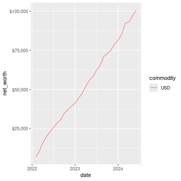
month_cutoff <- zoo::as.yearmon(Sys.Date()) - 2 / 12
compute_income <- function(df) {
    count_beans(df, "^Income", yearmon) %>%
        mutate(income = -amount) %>%
        select(-amount) %>%
        ungroup()
}
print_income <- function(df) {
    compute_income(df) %>%
        filter(yearmon >= month_cutoff) %>%
        spread(yearmon, income, fill = 0) %>%
        print_tibble_rows()
}
compute_expenses <- function(df) {
    count_beans(df, "^Expenses", yearmon) %>%
        mutate(expenses = amount) %>%
        select(-amount) %>%
        ungroup()
}
print_expenses <- function(df) {
    compute_expenses(df) %>%
        filter(yearmon >= month_cutoff) %>%
        spread(yearmon, expenses, fill = 0) %>%
        print_tibble_rows()
}
compute_total <- function(df) {
    full_join(
        compute_income(prune_coa(df)) %>% select(-account),
        compute_expenses(prune_coa(df)) %>% select(-account),
        by = c("yearmon", "commodity")
    ) %>%
        mutate(
            income = ifelse(is.na(income), 0, income),
            expenses = ifelse(is.na(expenses), 0, expenses),
            net = income - expenses
        ) %>%
        gather(type, amount, -yearmon, -commodity)
}
print_total <- function(df) {
    compute_total(df) %>%
        filter(yearmon >= month_cutoff) %>%
        spread(yearmon, amount, fill = 0) %>%
        print_tibble_rows()
}
print_total(df)
## # A tibble: 3 × 5
## commodity type `Apr 2026` `May 2026` `Jun 2026`
## <chr> <chr> <dbl> <dbl> <dbl>
## 1 USD expenses 7428. 7397. 2347.
## 2 USD income 10479. 10623. 5362.
## 3 USD net 3051. 3226. 3015.print_income(prune_coa(df, 2))## # A tibble: 1 × 5
## account commodity `Apr 2026` `May 2026` `Jun 2026`
## <chr> <chr> <dbl> <dbl> <dbl>
## 1 Income:US USD 10479. 10623. 5362.print_expenses(prune_coa(df, 2))## # A tibble: 6 × 5
## account commodity `Apr 2026` `May 2026` `Jun 2026`
## <chr> <chr> <dbl> <dbl> <dbl>
## 1 Expenses:Financial USD 4 13.0 13.0
## 2 Expenses:Food USD 516. 492. 245.
## 3 Expenses:Health USD 194. 194. 96.9
## 4 Expenses:Home USD 2610. 2594. 0
## 5 Expenses:Taxes USD 3984. 3984. 1992.
## 6 Expenses:Transport USD 120 120 0print_income(df)## # A tibble: 4 × 5
## account commodity `Apr 2026` `May 2026` `Jun 2026`
## <chr> <chr> <dbl> <dbl> <dbl>
## 1 Income:US:BayBook:GroupTermLife USD 48.6 48.6 24.3
## 2 Income:US:BayBook:Match401k USD 1200 1200 600
## 3 Income:US:BayBook:Salary USD 9231. 9231. 4615.
## 4 Income:US:ETrade:PnL USD 0 144 123.print_expenses(df)## # A tibble: 19 × 5
## account commodity `Apr 2026` `May 2026` `Jun 2026`
## <chr> <chr> <dbl> <dbl> <dbl>
## 1 Expenses:Financial:Commissions USD 0 8.95 8.95
## 2 Expenses:Financial:Fees USD 4 4 4
## 3 Expenses:Food:Groceries USD 160. 206. 181.
## 4 Expenses:Food:Restaurant USD 356. 286. 64.4
## 5 Expenses:Health:Dental:Insurance USD 5.8 5.8 2.9
## 6 Expenses:Health:Life:GroupTermLife USD 48.6 48.6 24.3
## 7 Expenses:Health:Medical:Insurance USD 54.8 54.8 27.4
## 8 Expenses:Health:Vision:Insurance USD 84.6 84.6 42.3
## 9 Expenses:Home:Electricity USD 65 65 0
## 10 Expenses:Home:Internet USD 79.9 80.1 0
## 11 Expenses:Home:Phone USD 65.4 48.7 0
## 12 Expenses:Home:Rent USD 2400 2400 0
## 13 Expenses:Taxes:Y2026:US:CityNYC USD 350. 350. 175.
## 14 Expenses:Taxes:Y2026:US:Federal USD 2126. 2126. 1063.
## 15 Expenses:Taxes:Y2026:US:Medicare USD 213. 213. 107.
## 16 Expenses:Taxes:Y2026:US:SDI USD 2.24 2.24 1.12
## 17 Expenses:Taxes:Y2026:US:SocSec USD 563. 563. 282.
## 18 Expenses:Taxes:Y2026:US:State USD 730. 730. 365.
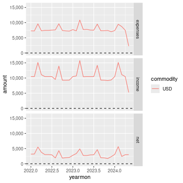
## 19 Expenses:Transport:Tram USD 120 120 0And here is a plot of income, expenses, and net income over time:
ggplot(
    compute_total(df),
    aes(x = yearmon, y = amount, group = commodity, colour = commodity)
) +
    facet_grid(type ~ .) +
    geom_line() +
    geom_hline(yintercept = 0, linetype = "dashed") +
    scale_x_continuous() +
    scale_y_continuous(labels = scales::comma)