

phylospatial is an R package for spatial phylogenetics:
mapping and analyzing biodiversity in a way that accounts for the
evolutionary relationships among taxa. The package is built around the
“phylogenetic diversity” family of metrics, which count each clade or
branch segment on the phylogeny rather than giving primacy to the
terminal species. It covers the full workflow, from building data sets
to mapping diversity and endemism, testing significance against null
models, comparing communities, delineating bioregions, and setting
conservation priorities. It is designed to be flexible:
terra), polygons or points (sf), or
occurrence records converted to a grid with ps_grid().
Results come back as maps ready to plot.vegan and nullcat (including stratified
algorithms designed for quantitative data), custom functions, and
spatially constrained null models that test whether sites are unusual
relative to their neighbors.# install the package from CRAN:
install.packages("phylospatial")
# or the development version from GitHub:
remotes::install_github("matthewkling/phylospatial")Analyses start from a phylospatial object, created by
phylospatial() from a community data set (a
SpatRaster or sf object with a layer or column
per taxon, or a site-by-taxon matrix) and a phylogeny. If your data are
occurrence points, ps_grid() converts them to a raster data
set first. The package includes an example data set of occurrence
probabilities for 443 moss species across California, along with their
phylogeny, which we’ll use here:
library(phylospatial)
library(terra)

ps <- moss()
ps
#> `phylospatial` object
#>   - 884 lineages across 527 occupied sites (1116 total)
#>   - community data type: probability
#>   - branch length rescaling: sum1
#>   - site weights: equal
#>   - spatial data class: SpatRaster
#>   - dissimilarity data: none
See vignette("phylospatial-data") for details on
constructing data sets.
ps_diversity() calculates a suite of richness,
divergence, and regularity metrics, including phylogenetic diversity
(PD) and phylogenetic endemism (PE):
div <- ps_diversity(ps, metric = c("PD", "PE"))
plot(div, axes = FALSE)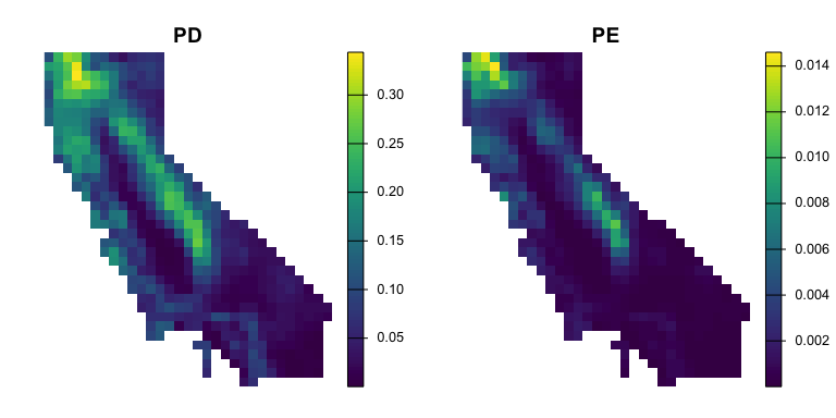
ps_rand() tests these metrics against a null model, and
ps_canape() uses the results to classify sites into centers
of neo- and paleo-endemism (CANAPE). There are a range of null model
algorithms available for different hypotheses and data types; see
vignette("alpha-diversity") for details. Here’s a quick
version with 1000 randomizations and a modest number of burn-in
iterations. Adding site_groups = ps_tile_groups(...) would
make the null model spatially constrained, comparing each site only to
its surroundings rather than to the whole study area.
rand <- ps_rand(ps, metric = c("PD", "PE", "CE", "RPE"), n_rand = 1000,
                fun = "quantize", method = "curvecat",
                transform = function(x) log10(x + 0.001),
                n_iter = 30000, n_cores = 8, progress = FALSE)

par(mfrow = c(1, 2))
plot(rand$qPD, axes = FALSE, main = "PD null quantile")

canape <- ps_canape(rand)
plot(canape, axes = FALSE, main = "CANAPE")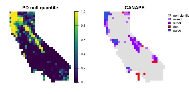
ps_dissim() computes various measures of phylogenetic
dissimilarity between sites, with options to partition it into turnover
and nestedness, weight lineages by endemism, and compare a focal site to
every other site (ps_dissim_focal()) or each site to itself
in another data set (ps_dissim_paired(), for example to
measure change over time). Dissimilarities feed into ordination
(ps_ordinate(), ps_rgb()) and
bioregionalization (ps_regions()), and can be used in a
wide range of analyses such as GDM and PERMANOVA tests. Here, sites with
similar colors on the left have similar lineage composition, and the map
on the right groups sites into four phylogenetic regions:
ps <- ps_add_dissim(ps, method = "sorensen", endemism = TRUE, normalize = TRUE)
rgb <- ps_rgb(ps, method = "cmds")
regions <- ps_regions(ps, k = 4, method = "average")

par(mfrow = c(1, 2))
plotRGB(rgb, scale = 1, smooth = FALSE, mar = c(0, 0, 2, 0),
        main = "Community ordination")
plot(regions, type = "classes", col = palette.colors(4, "Dark 2"), legend = FALSE,
     axes = FALSE, mar = c(0, 0, 2, 0), main = "Phylogenetic regions")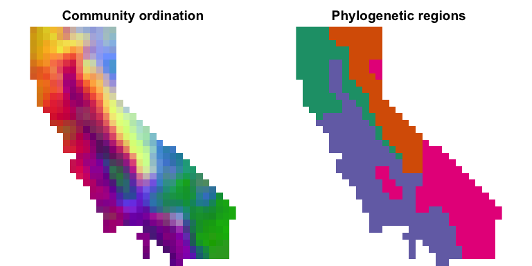
See vignette("beta-diversity") for more.
The package includes two approaches for computing optimal reserve
networks that protect evolutionary diversity while accounting for
existing protected areas, the cost of protection, and complementarity
among sites: ps_prioritize() finds a nested ranking of
sites, while ps_prioritizr() sets up a prioritizr problem that finds optimal
solutions for a given budget or target. ps_performance()
traces how conservation value accumulates along the ranking. Here, low
ranks (yellow) are the highest priorities for expanding California’s
protected areas to conserve moss lineages:
protection <- moss(data = "protection") # existing protection level of each site
cost <- 1 + log1p(moss(data = "popdens")) # population density as a proxy for cost
priority <- ps_prioritize(ps, init = protection, cost = cost, progress = FALSE)

rank_breaks <- c(0, 10, 25, 50, 100, 250, global(priority, "max", na.rm = TRUE)[[1]])
plot(priority, breaks = rank_breaks, col = rev(hcl.colors(6, "inferno")),
     axes = FALSE, plg = list(title = "priority rank"))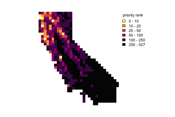
The package website has full documentation and four vignettes:
vignette("phylospatial-data"): constructing
phylospatial data sets from different types of data.vignette("alpha-diversity"): alpha diversity and
endemism metrics, null model randomization, and CANAPE.vignette("beta-diversity"): phylogenetic dissimilarity,
ordination, and regionalization.vignette("prioritization"): conservation prioritization
with ps_prioritize() and ps_prioritizr().To cite phylospatial in publications, please use:
Kling, M. (2025). phylospatial: an R package for spatial phylogenetic analysis with quantitative community data. Methods in Ecology and Evolution 16:1075–1083. DOI 10.1111/2041-210x.70056