The relliptical R package

The relliptical R package provides a function for random number generation from members of the truncated multivariate elliptical family of distributions, including truncated versions of the Normal, Student-t, Pearson type VII, Slash, Logistic, Kotz-type distributions, among others. The package also allows users to define custom elliptical distributions by explicitly specifying the density generating function. In addition, it computes the first- and second-order moments, including the covariance matrix, for some particular distributions. For more details, see (Valeriano, Galarza, and Matos 2023).

Next, we describe the main functions available in the package.

Random number generation

The function rtelliptical generates random observations from a truncated multivariate elliptical distribution with location parameter mu, scale matrix Sigma, and lower and upper truncation bounds specified by lower and upper, respectively. Sampling is performed using a Slice Sampling algorithm (Neal 2003) combined with Gibbs sampling steps (Robert and Casella 2010).

The argument dist specifies the truncated elliptical distribution to be used. The available options are Normal, t, PE, PVII, Slash, and CN, corresponding to the truncated Normal, Student-t, Power Exponential, Pearson type VII, Slash, and Contaminated Normal distributions, respectively.

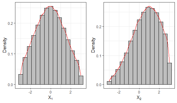
In the following example, we generate \(n = 10^5\) samples from a truncated bivariate Normal distribution.

library(relliptical)

# Sampling from the Truncated Normal distribution
set.seed(1234)
mu  = c(0, 1)
Sigma = matrix(c(3,0.6,0.6,3), 2, 2)
lower = c(-3, -3)
upper = c(3, 3)
sample1 = rtelliptical(n=1e5, mu, Sigma, lower, upper, dist="Normal")
head(sample1)
#>            [,1]       [,2]
#> [1,]  0.6643105  2.4005763
#> [2,] -1.3364441 -0.1756624
#> [3,] -0.1814043  1.7013605
#> [4,] -0.6841829  2.4750461
#> [5,]  2.0984490  0.1375868
#> [6,] -1.8796633 -1.2629126

library(ggplot2)
# Histogram and density for variable 1
f1 = ggplot(data.frame(sample1), aes(x=X1)) + 
  geom_histogram(aes(y=..density..), colour="black", fill="grey", bins=15) +
  geom_density(colour="red") + labs(x=bquote(X[1]), y="Density") + theme_bw()

# Histogram and density for variable 2
f2 = ggplot(data.frame(sample1), aes(x=X2)) + 
  geom_histogram(aes(y=..density..), colour="black", fill="grey", bins=15) +
  geom_density(colour="red") + labs(x=bquote(X[2]), y="Density") + theme_bw()

library(gridExtra)
grid.arrange(f1, f2, nrow=1)
#> Warning: The dot-dot notation (`..density..`) was deprecated in ggplot2 3.4.0.
#> ℹ Please use `after_stat(density)` instead.
#> This warning is displayed once every 8 hours.
#> Call `lifecycle::last_lifecycle_warnings()` to see where this warning was
#> generated.

This function also allows random number generation from truncated elliptical distributions not explicitly listed in the dist argument, by providing the density generating function (DGF) through either the expr or gFun arguments. The DGF must be a non-negative and strictly decreasing function on \((0, \infty)\). The simplest approach is to supply the DGF to the expr argument as a character string. The notation used in expr must be compatible with both the Ryacas package and the R evaluation environment. For example, for the DGF \(g(t)=e^{-t}\), the user should specify expr = "exp(-t)". The DGF expression must depend only on the variable \(t\); any additional parameters must be provided as fixed values. When a character expression is supplied via expr, the algorithm attempts to compute a closed-form expression for the inverse function of \(g(t)\). Since such an expression may not always exist, a warning message is issued whenever the inversion cannot be obtained analytically.

The following example generates random variates from a truncated bivariate Logistic distribution, whose DGF is given by \(g(t) = e^{-t}/(1+e^{-t})^2, t \geq 0\), see (Fang, Kotz, and Ng 2018).

# Sampling from the Truncated Logistic distribution
mu  = c(0, 0)
Sigma = matrix(c(1,0.70,0.70,1), 2, 2)
lower = c(-2, -2)
upper = c(3, 2)
# Sample autocorrelation with no thinning
set.seed(5678)
sample2 = rtelliptical(n=5000, mu, Sigma, lower, upper, expr="exp(-t)/(1+exp(-t))^2")
tail(sample2)
#>               [,1]       [,2]
#> [4995,] -0.1838654  0.1705458
#> [4996,] -0.6290305  0.7899355
#> [4997,] -0.7046777 -0.4168683
#> [4998,]  0.3311000  0.7107361
#> [4999,]  0.7265892  0.8110315
#> [5000,]  0.2588786 -0.2191296

If it is not possible to generate random samples by supplying a character expression to expr, the user may instead provide a custom R function via the gFun argument. By default, the inverse of this function is numerically approximated; however, for improved computational efficiency, the user may optionally supply the inverse function directly through the ginvFun argument. When gFun is provided, the arguments dist and expr are ignored.

In the following example, we generate samples from a truncated Kotz-type distribution, whose density generating function is given by

\[g(t) = t^{N-1} e^{-r t^s}, \quad t\geq 0, \quad r>0, \quad s>0, \quad 2N+p>2.\]

As required, this function is strictly decreasing when \((2-p)/2 < N \leq 1\); see (Fang, Kotz, and Ng 2018).

# Sampling from the Truncated Kotz-type distribution
set.seed(9876)
mu  = c(0, 0)
Sigma = matrix(c(1,0.70,0.70,1), 2, 2)
lower = c(-2, -2)
upper = c(3, 2)
sample4 = rtelliptical(n=1e4, mu, Sigma, lower, upper, gFun=function(t){ t^(-1/2)*exp(-2*t^(1/4)) })
f1 = ggplot(data.frame(sample4), aes(x=X1, y=X2)) + geom_point(size=0.50) +
     labs(x=expression(X[1]), y=expression(X[2]), subtitle="Kotz(2,1/4,1/2)") +
  theme_bw()

library(ggExtra)
ggMarginal(f1, type="histogram", fill="grey")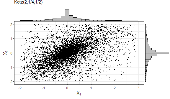

Since the sampling procedure relies on an MCMC-based algorithm, the generated observations may exhibit serial correlation. Therefore, it can be useful to examine autocorrelation function (ACF) plots to assess the dependence structure of the simulated samples. In the following, we analyze the sample generated from the bivariate Logistic distribution.

# Function for plotting the sample autocorrelation using ggplot2
acf.plot = function(samples){
  p = ncol(samples);   n = nrow(samples);   acf1 = list(p)
  for (i in 1:p){
    bacfdf = with(acf(samples[,i], plot=FALSE), data.frame(lag, acf))
    acf1[[i]] = ggplot(data=bacfdf, aes(x=lag,y=acf)) + geom_hline(aes(yintercept=0)) +
      geom_segment(aes(xend=lag, yend=0)) + labs(x="Lag", y="ACF", subtitle=bquote(X[.(i)])) +
      geom_hline(yintercept=c(qnorm(0.975)/sqrt(n),-qnorm(0.975)/sqrt(n)), colour="red", linetype="twodash") + theme_bw()
  }
  return (acf1)
}

grid.arrange(grobs=acf.plot(sample2), top="Sample ACF with no thinning", nrow=1)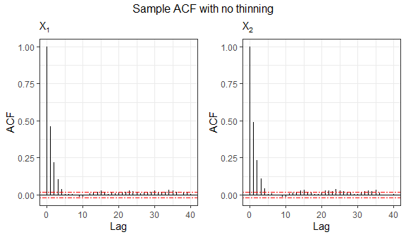

Autocorrelation can be reduced by specifying the thinning argument. The thinning factor decreases the dependence among sampled values in the Gibbs sampling process by retaining only every \(k\)-th iteration of the Markov chain. Naturally, this value must be an integer greater than or equal to 1.

# Sample autocorrelation with thinning = 3
set.seed(8768)
sample3 = rtelliptical(n=5000, mu, Sigma, lower, upper, dist=NULL, expr="exp(1)^(-t)/(1+exp(1)^(-t))^2", 
                       thinning=3)
grid.arrange(grobs=acf.plot(sample3), top="Sample ACF with thinning = 3", nrow=1)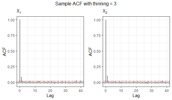

Mean vector and variance-covariance matrix

For this purpose, we use the function mvtelliptical(), which computes the mean vector and variance-covariance matrix for selected truncated multivariate elliptical distributions. The argumentdist specifies the distribution to be used and accepts the same options as before: Normal, t, PE, PVII, Slash, and CN. Moments for the truncated components are estimated using a Monte Carlo approach, while moments for the non-truncated components are obtained by exploiting properties of conditional expectation.

Next, we compute the moments of a random vector \(X\) following a truncated 3-variate Student-t distribution with \(\nu=0.8\) degrees of freedom. Two scenarios are considered: (i) a case with a single doubly truncated variable, and (ii) a case with two doubly truncated variables.

# Truncated Student-t distribution
set.seed(5678)
mu = c(0.1, 0.2, 0.3)
Sigma = matrix(data = c(1,0.2,0.3,0.2,1,0.4,0.3,0.4,1), nrow=length(mu), ncol=length(mu), byrow=TRUE)
# Example 1: considering nu = 0.80 and one doubly truncated variable
a = c(-0.8, -Inf, -Inf)
b = c(0.5, 0.6, Inf)
mvtelliptical(a, b, mu, Sigma, "t", 0.80)
#> $EY
#>             [,1]
#> [1,] -0.11001805
#> [2,] -0.54278399
#> [3,] -0.01119847
#> 
#> $EYY
#>            [,1]       [,2]       [,3]
#> [1,] 0.13761136 0.09694152 0.04317817
#> [2,] 0.09694152        NaN        NaN
#> [3,] 0.04317817        NaN        NaN
#> 
#> $VarY
#>            [,1]       [,2]       [,3]
#> [1,] 0.12550739 0.03722548 0.04194614
#> [2,] 0.03722548        NaN        NaN
#> [3,] 0.04194614        NaN        NaN

# Example 2: considering nu = 0.80 and two doubly truncated variables
a = c(-0.8, -0.70, -Inf)
b = c(0.5, 0.6, Inf)
mvtelliptical(a, b, mu, Sigma, "t", 0.80) # By default n=1e4
#> $EY
#>             [,1]
#> [1,] -0.08566441
#> [2,]  0.01563586
#> [3,]  0.19215627
#> 
#> $EYY
#>             [,1]        [,2]       [,3]
#> [1,] 0.126040187 0.005937196 0.01331868
#> [2,] 0.005937196 0.119761635 0.04700108
#> [3,] 0.013318682 0.047001083 1.14714388
#> 
#> $VarY
#>             [,1]        [,2]       [,3]
#> [1,] 0.118701796 0.007276632 0.02977964
#> [2,] 0.007276632 0.119517155 0.04399655
#> [3,] 0.029779636 0.043996554 1.11021985

As observed in the first scenario, some elements of the variance-covariance matrix are reported as NaN. These correspond to cases in which the associated moments do not exist (note that some elements of the variance-covariance matrix may exist while others do not). It is well known that, for an untruncated Student-t distribution, the second moment exists only when \(\nu > 2\). However, as shown by (Galarza et al. 2022), this condition can be relaxed when an increasing number of dimensions are subject to finite truncation limits.

It is also worth noting that the Student-t distribution with \(\nu > 0\) degrees of freedom is a special case of the Pearson type VII distribution with parameters \(m > p/2\) and \(\nu^* > 0\) obtained by setting \(m = (\nu+p)/2\) and \(\nu^* = \nu\).

Finally, for comparison purposes, we compute the moments of a truncated Pearson type VII distribution with parameters \(\nu^* = \nu = 0.80\) and \(m = (\nu + 3)/2 = 1.90\), which is equivalent to the Student-t distribution considered above. As expected, the resulting moments are nearly identical.

# Truncated Pearson VII distribution
set.seed(9876)
a = c(-0.8, -0.70, -Inf)
b = c(0.5, 0.6, Inf)
mu = c(0.1, 0.2, 0.3)
Sigma = matrix(data = c(1,0.2,0.3,0.2,1,0.4,0.3,0.4,1), nrow=length(mu), ncol=length(mu), byrow=TRUE)
mvtelliptical(a, b, mu, Sigma, "PVII", c(1.90,0.80), n=1e6) # n=1e6 more precision
#> $EY
#>             [,1]
#> [1,] -0.08558130
#> [2,]  0.01420611
#> [3,]  0.19166895
#> 
#> $EYY
#>             [,1]        [,2]       [,3]
#> [1,] 0.128348258 0.006903655 0.01420704
#> [2,] 0.006903655 0.121364742 0.04749544
#> [3,] 0.014207043 0.047495444 1.15156461
#> 
#> $VarY
#>             [,1]        [,2]       [,3]
#> [1,] 0.121024099 0.008119433 0.03061032
#> [2,] 0.008119433 0.121162929 0.04477257
#> [3,] 0.030610322 0.044772574 1.11482763

References

mirror server hosted at Truenetwork, Russian Federation.