Fitting topic models (and simulating text
data) with tmfast
Dan Hicks hicks.daniel.j@gmail.com
In this vignette, we demonstrate a basic workflow using
tmfastto fit topic models. We also show how the generators
included in the package can be used to create simulated text data. The
vignette assumes you’re already familiar with topic models, and
specifically the latent dirichlet allocation (LDA) data generation
model, along with PCA and varimax. The tmfast package was
inspired by Rohe and Zeng (2020), who
provide the mathematical justification for treating topic modeling as
varimax-rotated PCA, but somewhat finicky and incomplete software for
actually fitting models using this approach.
library(dplyr)
library(tidyr)
library(tibble)
library(purrr)
## Warning: package 'purrr' was built under R version 4.5.2library(stringr)
library(ggplot2)
library(lpSolve) # For matching fitted and trust topics
library(tictoc) # For checking timing
library(tmfast)
library(stm) # Used for comparison## stm v1.3.8 successfully loaded. See ?stm for help.
## Papers, resources, and other materials at structuraltopicmodel.comlibrary(tidytext) # Used for stm tidiersSimulated text data
Simulation parameters
We create simulated text data following the data-generating process assumed by LDA. Specifically, each document will be generated from one of several “journals.” Each journal corresponds to a topic, and vice versa, in that documents from journal \(j\) will tend to have a much greater mixture (probably) of topic \(j\) than the other topics.
We first specify the number of topics/journals k, and
the number of documents to draw from each journal Mj, for a
total of M = Mj * k documents in the corpus. We also
specify the length of the vocabulary (total unique words) as a multiple
of the total number of documents M. Document lengths are
generated using a negative binomial distribution, using the size-mean
parameterization. Per ?NegBinomial, the standard deviation
of document lengths in this parameterization is \(\sqrt{\mu +
\frac{\mu^2}{\mathrm{size}}}\)
k = 10 # Num. topics / journals
Mj = 100 # Num. documents per journal
M = Mj * k # Total corpus size
vocab = M # Vocabulary length

## Negative binomial distribution of doc lengths
size = 10 # Size and mean
mu = 300
sqrt(mu + mu^2 / size) # Resulting SD of document sizes
## [1] 96.43651## Dirichlet distributions for topic-docs and word-topics
topic_peak = .8
topic_scale = 10
word_beta = 0.1Because the simulations involve drawing samples using a RNG, we first set a seed.
set.seed(2022 - 06 - 19)Draw true topic distributions
We first generate the true topic-document distributions \(p(\theta = t | \mathrm{doc}_m)\), often
simply called \(\theta\) or \(\gamma\). In this vignette we use \(\theta\) for the true distribution and
\(\gamma\) for the fitted distribution
in the topic model. Each document’s \(\theta\) is sampled from a Dirichlet
distribution (rdirichlet()), with the parameter \(\mathbf{\alpha}\) corresponding to the
document’s journal \(j\). The variable
theta is a M by k matrix;
theta_df is a tidy representation with columns
doc, topic, and prob. The
visualization confirms that documents are generally most strongly
associated with the corresponding topics, though with some noise.
## Journal-specific alpha, with a peak value (.8 by default) and uniform otherwise
theta = map(
      1:k,
      ~ rdirichlet(
            Mj,
            peak_alpha(k, .x, peak = topic_peak, scale = topic_scale)
      )
) |>
      reduce(rbind)

theta_df = theta |>
      as_tibble(rownames = 'doc', .name_repair = tmfast:::make_colnames) |>
      mutate(doc = as.integer(doc)) |>
      pivot_longer(starts_with('V'), names_to = 'topic', values_to = 'prob')

ggplot(theta_df, aes(doc, topic, fill = prob)) +
      geom_tile()
Draw true word distributions
Next we generate the true word-topic distributions \(p(\phi = w | \theta = t)\), often designed as either \(\phi\) or \(\beta\). We use \(\phi\) for the true distribution and \(\beta\) for the fitted distribution. We sample these distributions from a symmetric Dirichlet distribution over the length of the vocabulary with \(\alpha = .01\). Tile and Zipfian (probability vs. rank on a log-log scale) plots confirm these distributions are working correctly.
## phi_j:  Word distribution for topic j
phi = rdirichlet(k, word_beta, k = vocab)

## Word distributions
phi |>
      as_tibble(rownames = 'topic', .name_repair = tmfast:::make_colnames) |>
      pivot_longer(starts_with('V'), names_to = 'word', values_to = 'prob') |>
      ggplot(aes(topic, word, fill = (prob))) +
      geom_tile() +
      scale_y_discrete(breaks = NULL)
## Zipf's law
phi |>
      as_tibble(rownames = 'topic', .name_repair = \(x) {
            (str_c('word', 1:vocab))
      }) |>
      pivot_longer(
            starts_with('word'),
            names_to = 'word',
            values_to = 'prob'
      ) |>
      group_by(topic) |>
      mutate(rank = rank(desc(prob))) |>
      arrange(topic, rank) |>
      filter(rank < vocab / 2) |>
      ggplot(aes(rank, prob, color = topic)) +
      geom_line() +
      scale_x_log10() +
      scale_y_log10()
Document lengths
Again, document lengths are drawn from a negative binomial distribution.
## N_i:  Length of document i
N = rnbinom(M, size = size, mu = mu)
summary(N)
## Min. 1st Qu. Median Mean 3rd Qu. Max.
## 93.0 240.8 300.5 308.6 364.5 774.0sd(N)## [1] 95.1555hist(N)
Draw corpus
Finally we draw the corpus, the observed word counts for each
document. This is the most time-consuming step in this script, much
slower than actually fitting the topic model. Experimenting with this
simulation, we found that log1p() scaling of the word
counts produced better results than other scaling techniques (eg,
dividing by the total length of each document, scaling words by their
standard deviation) for accounting for radical differences in document
length.
tic()
corpus = draw_corpus(N, theta, phi)
toc()
## 7.912 sec elapseddtm = mutate(corpus, n = log1p(n))Fit the topic model
Fitting the topic model is extremely fast. Note that we can request
multiple numbers of topics in a single call. Under the hood, we first
cast the document-term matrix (which is already in a sparse
representation) to a sparse matrix. Then we extract the maximum number
of desired principal components using
irlba::prcomp_irlba(), centering but not scaling the logged
word counts. (Experiments with this simulation indicated that scaling
makes it more difficult to construct probability distributions later.)
irlba implements an extremely efficient
algorithm for partial singular value decompositions of large sparse
matrices. Next we use stats::varimax() to construct a
preliminary varimax rotation of the principal components. Because the
direction of factors is arbitrary as far as varimax is concerned, but
meaningful when we convert things to probability distributions, we check
the skew of each factor’s loadings in the preliminary fit, and reverse
the factors with negative skew (long left tails).1
tic()
fitted = tmfast(dtm, c(2, 3, k, 2 * k))
toc()
## 0.224 sec elapsedThe object returned by tmfast() has a simple structure.
totalvar and sdev come from the PCA step,
giving the total variance across all feature variables and the standard
deviation of each extracted principal component. (Note that these PCs do
not generally correspond to the varimax-rotated factors/topics.)
n contains the sizes (number of factors/topics) fitted for
the models, and varimaxes contains the varimax fit for each
value of n. The varimax objects each contain three
matrices, the rotated loadings (word-topics), the rotation
matrix rotmat, and the rotated scores
(document-topics).
str(fitted, max.level = 2L)## List of 10
## $ totalvar: num 138
## $ sdev : num [1:20] 3.26 3.06 3.01 2.97 2.93 ...
## $ rows : chr [1:1000] "1" "2" "3" "4" ...
## $ cols : chr [1:999] "5" "7" "8" "11" ...
## $ center : Named num [1:999] 0.4016 0.0943 0.4254 0.2396 0.4093 ...
## ..- attr(*, "names")= chr [1:999] "5" "7" "8" "11" ...
## $ scale : logi FALSE
## $ x :Formal class 'dgCMatrix' [package "Matrix"] with 6 slots
## $ rotation: num [1:999, 1:20] -0.00112 0.02725 0.01223 0.00457 -0.00883 ...
## ..- attr(*, "dimnames")=List of 2
## $ n : num [1:4] 2 3 10 20
## $ varimax :List of 4
## ..$ 2 :List of 3
## ..$ 3 :List of 3
## ..$ 10:List of 3
## ..$ 20:List of 3
## - attr(*, "class")= chr [1:3] "tmfast" "varimaxes" "list"str(fitted$varimax$`10`)## List of 3
## $ loadings: num [1:999, 1:10] -0.0479 0.1025 0.0436 -0.0414 -0.0505 ...
## ..- attr(*, "dimnames")=List of 2
## .. ..$ : chr [1:999] "5" "7" "8" "11" ...
## .. ..$ : NULL
## $ rotmat : num [1:10, 1:10] 0.784 0.2228 0.23 0.0823 -0.3342 ...
## $ scores : num [1:1000, 1:10] -0.384 -0.137 -0.253 -0.298 -0.388 ...
## ..- attr(*, "dimnames")=List of 2
## .. ..$ : chr [1:1000] "1" "2" "3" "4" ...
## .. ..$ : NULLBecause the model contains a sdev component,
screeplot() works out of the box. Note that the first \(k\) PCs have much higher variance than the
others, and often the \(k\)th PC is
somewhat lower than the first \(k-1\).
This reflects the highly simplified structure of the simulated data.
Real datasets often have a much more gradual decline in the screeplot,
likely reflecting the complex hierarchy of topics in actual
documents.
screeplot(fitted)
It’s also straightforward to calculate the share of total variance covered by successive principal components. Experimenting with this simulation, when some documents are much larger than others, \(k\) PCs might cover less than half of the total variance. In this case it covers about 65%. Again, note that the rotated varimax factors don’t correspond to the principal components; but the total covered variance remains the same.
## Variance coverage?
cumsum(fitted$sdev^2) / fitted$totalvar
## [1] 0.07689789 0.14466433 0.21018176 0.27420309 0.33636478 0.39492291
## [7] 0.45196354 0.50563725 0.55705654 0.57380104 0.57606900 0.57828256
## [13] 0.58048004 0.58264465 0.58479395 0.58691426 0.58902127 0.59107016
## [19] 0.59311409 0.59514063data.frame(
PC = 1:length(fitted$sdev),
cum_var = cumsum(fitted$sdev^2) / fitted$totalvar
) |>
ggplot(aes(PC, cum_var)) +
geom_line() +
geom_point()
Fitting a conventional topic model (stm)
For comparison, we’ll also fit a conventional topic model using the
stm package. To address the challenge of picking a number
of topics, it will conduct a topic estimation process when passed
K = 0. With the simulation parameters and the random seed
used here, this process takes almost 12 seconds and produces a model
with 36 topics. We therefore do not automatically run the next
chunk.
tic()
corpus |>
      cast_sparse(doc, word, n) |>
      stm(K = 0, verbose = FALSE)
toc()
Setting K = k gives us a fitted topic model in a few
seconds, about an order of magnitude slower than
tmfast().
tic()
fitted_stm = corpus |>
      cast_sparse(doc, word, n) |>
      stm(K = k, verbose = FALSE)
toc()
## 1.691 sec elapsedAssessing accuracy
Using simulated data with true word-topic and topic-document distributions lets us check the accuracy of varimax-based topic models. Here we’ll develop a method proposed by Malaterre and Lareau (2022), comparing distributions using Hellinger distance. For discrete probability distributions \(p, q\) over the same space \(X\), the Hellinger distance is given by \[ d(p,q) = \frac{1}{\sqrt{2}} \sqrt{\sum_{x \in X} (\sqrt{p(x)} - \sqrt{q(x)})^2} = \frac{1}{\sqrt{2}} \lVert \sqrt p - \sqrt q \rVert_2.\] The last equation means that the Hellinger distance is the Euclidean (\(L^2\)-norm) distance between the square roots of the distributions. Some authors working with topic models sometimes compare distributions using the \(L^2\)-norm of the distributions themselves, without the square root. But this approach is flawed, since probability distributions can have different lengths in the \(L^2\) norm. (For example, the distribution \(\left< 1, 0\right>\) has \(L^2\) length 1, while \(\left< \frac{1}{2}, \frac{1}{2} \right>\) has \(L^2\) length approximately 1.19.)2
Hellinger distance satisfies the equation \[ 1 - d^2(p, q) = \sum_{x \in X} \sqrt{p(x)q(x)}.
\] When working with topic models, we’re interested in pairwise
sets of Hellinger distances, either between all pairs of distributions
from a single set (for example, the topic distributions for each
document, as used in “discursive space” analysis [cite and
xref]) or two sets (for example, comparing fitted vs. true
word-topic distributions, as in this section). Working with two sets of
distributions \(P = \{p_i | i \in I\}\)
and \(Q = \{q_j | j \in J\}\), the
right-hand side of the last equation is equivalent to a matrix
multiplication.3 The hellinger() function
provides S3 methods for calculating Hellinger pairwise distances given a
single dataframe, single matrix, or two dataframes or matrices.
First, however, we need to extract the word-topic distributions.
tmfast provides a tidy() method, following the
pattern of the topicmodel tidiers in tidytext. Unlike other
topic models, tmfast objects can contain models for
multiple different values of \(k\)
(numbers of topics). So, in the second argument to tidy(),
we need to specify which number of topics we want. The third argument
specifies the desired set of distributions, either word-topics
('beta') or topic-documents ('gamma').
## beta: fitted varimax loadings, transformed to probability distributions
beta = tidy(fitted, k, 'beta')
Word-topic distributions correspond to the varimax factor loadings. These loadings can take any real value, so we use softmax (\(e^x / \sum e^x\)) within each factor (topic) to transform them to a probability distribution. The Zipfian plot below compares the fitted and true word-topic distributions. Consistently across experiments with this simulation, the softmax-transformed fitted distributions are radically flatter than the true ones.
## For convenience, arrange phi in a tidy-like format
phi_tidy = phi |>
      t() |>
      as_tibble(
            rownames = 'token',
            .name_repair = tmfast:::make_colnames
      ) |>
      pivot_longer(
            starts_with('V'),
            names_to = 'topic',
            values_to = 'beta'
      ) |>
      mutate(beta_rn = beta) |>
      mutate(type = 'true')

## Compare Zipfian distributions
bind_rows(
      mutate(beta, type = 'fitted'),
      phi_tidy
) |>
      group_by(type, topic) |>
      mutate(rank = rank(desc(beta))) |>
      arrange(type, topic, rank) |>
      filter(rank < vocab / 2) |>
      ggplot(aes(rank, beta, color = type, group = interaction(topic, type))) +
      geom_line() +
      scale_y_log10() +
      scale_x_log10()
This flatter distribution corresponds to greater entropy. In this simulation, the entropy of the true distributions slightly over 7 bits, while the fitted distributions are nearly 10 bits.
phi_tidy |>
      group_by(topic) |>
      summarize(entropy = entropy(beta))
## # A tibble: 10 × 2
## topic entropy
## <chr> <dbl>
## 1 V01 7.23
## 2 V02 7.26
## 3 V03 7.36
## 4 V04 7.12
## 5 V05 7.34
## 6 V06 7.15
## 7 V07 7.12
## 8 V08 7.25
## 9 V09 7.26
## 10 V10 7.30beta |>
group_by(topic) |>
summarize(entropy = entropy(beta))## # A tibble: 10 × 2
## topic entropy
## <chr> <dbl>
## 1 V01 9.96
## 2 V02 9.96
## 3 V03 9.96
## 4 V04 9.96
## 5 V05 9.96
## 6 V06 9.96
## 7 V07 9.96
## 8 V08 9.96
## 9 V09 9.96
## 10 V10 9.96Renormalizing fitted distributions
To mitigate the tendency of tmfast to produce
distributions that are too flat, when extracting probability
distributions with tidy() we add an optional
renormalization step.
Given a discrete probability distribution \(P\) with components \(p_i\) and entropy \(H\), and a parameter \(\beta\), we can define a new distribution \(P'\) with components
\[ p'_i = \frac{p_i^\beta}{\sum_i p_i^\beta} = \frac{p_i^\beta}{Z}\]
which has entropy
\[ H' = \frac{1}{Z} \sum_i [p_i^\beta \beta \log p_i] - \log Z.\]
That is, we can choose an exponent \(\beta\) that renormalizes \(P\) to achieve a target entropy \(H'\). In LDA, the target entropy is the
expected entropy for the underlying Dirichlet prior, for either
word-topic or topic-document distributions (depending on which set of
probability distributions are being extracted). tmfast
provides convenience functions for calculating this expected
entropy.
Note how the expected entropy of the Dirichlet distribution used to draw \(\phi\) corresponds to the mean entropy of the word-topic distributions in \(\phi\) calculated above.
expected_entropy(word_beta, k = vocab)## [1] 7.262407In actual applications, where the Dirichlet prior is an idealization, setting the target entropy is an important researcher degree of freedom. It plays roughly the same role as choosing prior parameters in other topic modeling packages.
Since solving for the exponent in the equation for \(H'\) requires numerical optimization,
it’s inefficient to do this every time we call tidy(),
especially with the topic-document distributions for large corpora.
Instead, tmfast::target_power() is used to run this
optimization once, returning the mean target exponent, and we can use
this value in all future calls to tidy().
beta_power = target_power(
      tidy_df = beta,
      group_col = topic,
      p_col = beta,
      target_entropy = expected_entropy(word_beta, k = vocab)
)
beta_power
## [1] 9.303478The result is a better approximation to the true word-topic distributions.
## Renormalized beta
beta_rn = tidy(fitted, k, 'beta', exponent = beta_power)

## Entropies after renormalization
beta_rn |>
      group_by(topic) |>
      summarize(entropy = entropy(beta))
## # A tibble: 10 × 2
## topic entropy
## <chr> <dbl>
## 1 V01 6.86
## 2 V02 7.16
## 3 V03 7.05
## 4 V04 7.36
## 5 V05 7.37
## 6 V06 6.46
## 7 V07 7.60
## 8 V08 7.72
## 9 V09 7.74
## 10 V10 7.01## Compare Zipfian distributions
bind_rows(
mutate(beta_rn, type = 'fitted'),
phi_tidy
) |>
group_by(type, topic) |>
mutate(rank = rank(desc(beta))) |>
arrange(type, topic, rank) |>
filter(rank < vocab / 2) |>
ggplot(aes(rank, beta, color = type, group = interaction(topic, type))) +
geom_line() +
scale_y_log10() +
scale_x_log10()
Topic alignment
The Zipfian distribution plot doesn’t tell us which fitted topics
might correspond to which true topics. For that, following Malaterre and
Lareau, we’ll use pairwise Hellinger distances. There’s one
complication, however. The parameters chosen for this simulation
typically end up not drawing some of the words from the vocabulary, and
they don’t end up in the same order as the true word-topic matrix
phi. Fortunately words are represented as the integers
1:vocab, so it’s relatively painless to put them back in
order and fill in the gaps (setting the probability for the missing
words to be 0 across all topics). In the pipe below, we first fix these
issues with the words, widen the long dataframe, convert it to a matrix,
and then calculate pairwise Hellinger distances with the true word-topic
matrix phi.
## Hellinger distance of word-topic distributions
beta_mx = beta_rn |>
      ## Fix order of words
      mutate(token = as.integer(token)) |>
      arrange(token) |>
      ## And dropped words
      complete(token = 1:vocab, topic, fill = list(beta = 0)) |>
      pivot_wider(
            names_from = 'topic',
            values_from = 'beta',
            values_fill = 0,
            names_sort = TRUE
      ) |>
      # select(-`NA`) |>
      ## Coerce to matrix
      column_to_rownames('token') |>
      as.matrix()

hellinger(phi, t(beta_mx))
## V01 V02 V03 V04 V05 V06 V07
## [1,] 0.8264397 0.3757451 0.8398115 0.8315508 0.8029694 0.8424367 0.8187739
## [2,] 0.8338319 0.8174157 0.8346582 0.8248563 0.3850327 0.8510000 0.8013987
## [3,] 0.8434356 0.8062143 0.8200851 0.7927524 0.8109665 0.8233865 0.8072406
## [4,] 0.8647348 0.8406944 0.3755762 0.8263752 0.8217148 0.8377416 0.8341385
## [5,] 0.8244662 0.8192211 0.8181999 0.8188743 0.8070537 0.8346530 0.3793745
## [6,] 0.8482153 0.8386428 0.8051109 0.8079935 0.8150622 0.4000049 0.8037098
## [7,] 0.3767702 0.8365954 0.8491229 0.8106023 0.8133025 0.8618251 0.8110033
## [8,] 0.8409601 0.8190504 0.8437947 0.8155441 0.8171708 0.8396975 0.7974495
## [9,] 0.8439760 0.8279738 0.8291009 0.3909809 0.8184996 0.8303775 0.8100712
## [10,] 0.8468421 0.8294605 0.8321105 0.8154655 0.8019464 0.8339808 0.7913169
## V08 V09 V10
## [1,] 0.8178268 0.7930654 0.8214260
## [2,] 0.8135240 0.8038809 0.8282732
## [3,] 0.8113352 0.3834189 0.8366152
## [4,] 0.8186043 0.8156843 0.8272566
## [5,] 0.7876117 0.7818178 0.8218345
## [6,] 0.8030155 0.8101810 0.8276411
## [7,] 0.8145190 0.8192976 0.8329151
## [8,] 0.7955823 0.8236388 0.4050044
## [9,] 0.8015495 0.7999218 0.8261243
## [10,] 0.3937114 0.8178691 0.8153404In this distance matrix, the rows are the true topics and the columns
are the fitted topics. Low values include that the topics are closer to
each other. It’s clear that the topics don’t match up perfectly —
typically the minimum in each row is about 0.38 — but there is a clear
minimum. We treat this as a linear assignment problem, which is solved
rapidly using the lpSolve package. The solution — which
matches true to fitted topics — can then be used as a rotation with both
the loadings and scores (topic-document distributions). After rotating,
the true-fitted pairs are on the diagonal of the Hellinger distance
matrix, making it easy to extract and summarize the quality of the
fit.
## Use lpSolve to match fitted topics to true topics
dist = hellinger(phi, t(beta_mx))
soln = lp.assign(dist)
soln$solution
## [,1] [,2] [,3] [,4] [,5] [,6] [,7] [,8] [,9] [,10]
## [1,] 0 1 0 0 0 0 0 0 0 0
## [2,] 0 0 0 0 1 0 0 0 0 0
## [3,] 0 0 0 0 0 0 0 0 1 0
## [4,] 0 0 1 0 0 0 0 0 0 0
## [5,] 0 0 0 0 0 0 1 0 0 0
## [6,] 0 0 0 0 0 1 0 0 0 0
## [7,] 1 0 0 0 0 0 0 0 0 0
## [8,] 0 0 0 0 0 0 0 0 0 1
## [9,] 0 0 0 1 0 0 0 0 0 0
## [10,] 0 0 0 0 0 0 0 1 0 0hellinger(phi, soln$solution %*% t(beta_mx))## [,1] [,2] [,3] [,4] [,5] [,6] [,7]
## [1,] 0.3757451 0.8029694 0.7930654 0.8398115 0.8187739 0.8424367 0.8264397
## [2,] 0.8174157 0.3850327 0.8038809 0.8346582 0.8013987 0.8510000 0.8338319
## [3,] 0.8062143 0.8109665 0.3834189 0.8200851 0.8072406 0.8233865 0.8434356
## [4,] 0.8406944 0.8217148 0.8156843 0.3755762 0.8341385 0.8377416 0.8647348
## [5,] 0.8192211 0.8070537 0.7818178 0.8181999 0.3793745 0.8346530 0.8244662
## [6,] 0.8386428 0.8150622 0.8101810 0.8051109 0.8037098 0.4000049 0.8482153
## [7,] 0.8365954 0.8133025 0.8192976 0.8491229 0.8110033 0.8618251 0.3767702
## [8,] 0.8190504 0.8171708 0.8236388 0.8437947 0.7974495 0.8396975 0.8409601
## [9,] 0.8279738 0.8184996 0.7999218 0.8291009 0.8100712 0.8303775 0.8439760
## [10,] 0.8294605 0.8019464 0.8178691 0.8321105 0.7913169 0.8339808 0.8468421
## [,8] [,9] [,10]
## [1,] 0.8214260 0.8315508 0.8178268
## [2,] 0.8282732 0.8248563 0.8135240
## [3,] 0.8366152 0.7927524 0.8113352
## [4,] 0.8272566 0.8263752 0.8186043
## [5,] 0.8218345 0.8188743 0.7876117
## [6,] 0.8276411 0.8079935 0.8030155
## [7,] 0.8329151 0.8106023 0.8145190
## [8,] 0.4050044 0.8155441 0.7955823
## [9,] 0.8261243 0.3909809 0.8015495
## [10,] 0.8153404 0.8154655 0.3937114hellinger(phi, soln$solution %*% t(beta_mx)) |>
diag() |>
summary()## Min. 1st Qu. Median Mean 3rd Qu. Max.
## 0.3756 0.3774 0.3842 0.3866 0.3930 0.4050And we do the same thing with the conventional topic model. It performs somewhat better, with a median Hellinger distance of about 0.08. But again, fitting this model is significantly slower.
beta_stm_mx = tidy(fitted_stm, matrix = 'beta') |>
      ## Fix order of words
      mutate(term = as.integer(term)) |>
      arrange(term) |>
      ## And dropped words
      complete(term = 1:vocab, topic, fill = list(beta = 0)) |>
      pivot_wider(
            names_from = 'topic',
            values_from = 'beta',
            values_fill = 0,
            names_sort = TRUE
      ) |>
      # select(-`NA`) |>
      ## Coerce to matrix
      column_to_rownames('term') |>
      as.matrix()

hellinger(phi, t(beta_stm_mx))
## 1 2 3 4 5 6
## [1,] 0.08551309 0.84250822 0.84248081 0.88213456 0.87444893 0.87158481
## [2,] 0.84329982 0.85367764 0.08226138 0.87003915 0.85853149 0.86965052
## [3,] 0.84814586 0.08498166 0.84966319 0.85873081 0.83485510 0.87731318
## [4,] 0.88728389 0.86458833 0.87596785 0.08716286 0.86137815 0.90341308
## [5,] 0.86509991 0.84154855 0.84198045 0.86693014 0.85183939 0.85492694
## [6,] 0.89275256 0.85458013 0.87148757 0.83690612 0.84770566 0.89098313
## [7,] 0.87604584 0.87475679 0.86935792 0.89497551 0.86136570 0.08426198
## [8,] 0.86179696 0.88513645 0.87104983 0.87765103 0.85763363 0.88206881
## [9,] 0.88272457 0.84014143 0.86831191 0.85799772 0.09038414 0.86010657
## [10,] 0.88217497 0.87848728 0.86296462 0.86880294 0.85154928 0.87344610
## 7 8 9 10
## [1,] 0.8505157 0.86539554 0.87856776 0.86805817
## [2,] 0.8615900 0.87026329 0.85983013 0.85353576
## [3,] 0.8822492 0.85827128 0.87289289 0.84502057
## [4,] 0.8729586 0.83661049 0.86684066 0.87271754
## [5,] 0.8460363 0.86047844 0.83835726 0.07902305
## [6,] 0.8628231 0.08880366 0.85411796 0.86252219
## [7,] 0.8747440 0.89536041 0.86677815 0.85727482
## [8,] 0.0926754 0.87054303 0.84452963 0.85300520
## [9,] 0.8517883 0.85313257 0.85250714 0.85785593
## [10,] 0.8460104 0.85587071 0.09097124 0.84596307rotation_stm = hellinger(phi, t(beta_stm_mx)) |>
lp.assign() |>
magrittr::extract2('solution')
hellinger(phi, rotation_stm %*% t(beta_stm_mx)) |>
diag() |>
summary()## Min. 1st Qu. Median Mean 3rd Qu. Max.
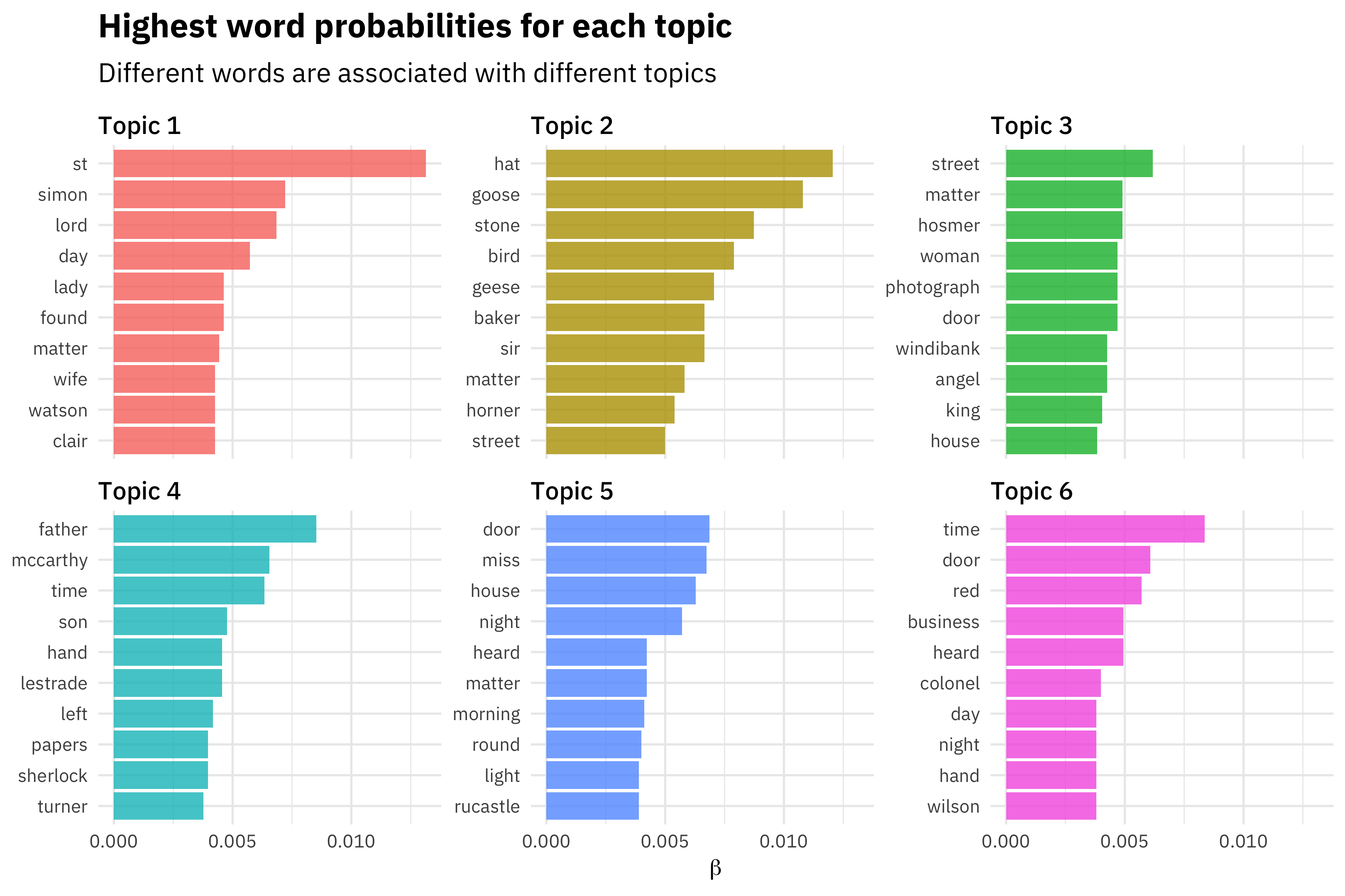
## 0.07902 0.08444 0.08634 0.08660 0.08999 0.09268The tidied word-topic distributions can be used in standard ways for further analysis, such as a Silge plot of the highest probability words for each topic. But because the “words” in this simulation are just integers, and not semantically meaningful, we don’t construct such a plot here.
Topic-document distributions
We extract topic-document distributions using the same
tidy() function, specifying the matrix gamma
and including the rotation above to align the fitted and true topics. As
with the loadings, the topic-document scores are transformed to
probability distributions using softmax and need to be renormalized.
## Example Dirichlet distribution used in drawing the true topic-document distributions
peak_alpha(k, 1, topic_peak, topic_scale)
## [1] 8.0000000 0.2222222 0.2222222 0.2222222 0.2222222 0.2222222 0.2222222
## [8] 0.2222222 0.2222222 0.2222222expected_entropy(peak_alpha(k, 1, topic_peak, topic_scale))## [1] 0.997604## Renormalization exponent
gamma_power = tidy(fitted, k, 'gamma') |>
target_power(
document,
gamma,
expected_entropy(peak_alpha(k, 1, topic_peak, topic_scale))
)
gamma_power## [1] 1.371585gamma_df = tidy(
fitted,
k,
'gamma',
rotation = soln$solution,
exponent = gamma_power
)## ℹ Rotating scoresgamma_df## # A tibble: 10,000 × 3
## document topic gamma
## <chr> <chr> <dbl>
## 1 1 V01 0.944
## 2 1 V02 0.00925
## 3 1 V03 0.00775
## 4 1 V04 0.00543
## 5 1 V05 0.00580
## 6 1 V06 0.00564
## 7 1 V07 0.00535
## 8 1 V08 0.00563
## 9 1 V09 0.00512
## 10 1 V10 0.00623
## # ℹ 9,990 more rowsTile and parallel coordinates plots can be used to visualize all of the topic-document distributions. These show that the varimax topic models successfully recover the overall association of each document’s journal with a distinctive topic.
gamma_df |>
      mutate(document = as.integer(document)) |>
      ggplot(aes(document, topic, fill = gamma)) +
      geom_raster() +
      scale_x_continuous(breaks = NULL)
gamma_df |>
      mutate(
            document = as.integer(document),
            journal = (document - 1) %/% Mj + 1
      ) |>
      ggplot(aes(topic, gamma, group = document, color = as.factor(journal))) +
      geom_line(alpha = .25) +
      facet_wrap(vars(journal), scales = 'free_x') +
      scale_color_discrete(guide = 'none')
We can now assess accuracy of the topic-document distributions. Above
we used the hellinger() method for two matrices. The method
for two dataframes requires specifying the id, topic, and probability
columns; see ?hellinger.data.frame. The tile plot shows
that the true and fitted topics are aligned (because we used the
rotation when extracting gamma_df above), and so again we
can get an overall summary from the diagonal. In the current simulation,
the mean Hellinger distance is 0.20.
hellinger(
      theta_df,
      id1 = doc,
      topics2 = gamma_df,
      id2 = document,
      prob2 = gamma,
      df = FALSE
) |>
      diag() |>
      summary()
## Min. 1st Qu. Median Mean 3rd Qu. Max.
## 0.05073 0.16551 0.20263 0.20395 0.23758 0.45066STM has a closer fit, with a mean Hellinger distance of 0.08.
fitted_stm_gamma = tidy(fitted_stm, matrix = 'gamma') |>
      pivot_wider(names_from = 'topic', values_from = 'gamma') |>
      column_to_rownames('document') |>
      as.matrix()

hellinger(theta, fitted_stm_gamma %*% t(rotation_stm)) |>
      diag() |>
      summary()
## Min. 1st Qu. Median Mean 3rd Qu. Max.
## 0.03216 0.07148 0.08638 0.08822 0.10260 0.19884Discursive space visualization using t-SNE and UMAP
Hicks (2021) proposed using topic models and Hellinger distance to
analyze the relative position of documents in “discursive space.” That
paper used the t-SNE dimension-reduction algorithm to produce a 2D
visualization of Hellinger distances. The UMAP algorithm is also
popular, and is believed to
do better than t-SNE at preserving global structure. tmfast
provides functions tsne() and umap() to
efficiently produce such visualizations. Note that the t-SNE algorithm
involves further random number draws (I believe to set the initial
positions of the points), so repeatedly running this next chunk will
produce superficially different visualizations.
tsne(fitted, k) |>
      mutate(journal = (as.integer(document) - 1) %/% Mj + 1) |>
      ggplot(aes(x, y, color = as.character(journal))) +
      geom_point() +
      labs(title = 't-SNE visualization')
umap(fitted, k, df = TRUE) |>
      mutate(journal = (as.integer(document) - 1) %/% Mj + 1) |>
      ggplot(aes(x, y, color = as.character(journal))) +
      geom_point() +
      labs(title = 'UMAP visualization')
Varimax is more often associated with factor analysis than PCA, because varimax-rotated basis vectors are no longer orthogonal. Unlike PCA, in topic modeling we don’t care about orthogonality. And unlike factor analysis, we’re not interested in dropping features (words) that don’t load substantially on exactly one factor (topic).↩︎
Cosine similarity is directly related to the \(L^2\)-norm, and has the same problem.↩︎
For \(P\), each row corresponds to the elementwise square root of one distribution \(\sqrt p_i\) and each column to one component \(x \in X\), i.e., a cell contains the value \(\sqrt{p_i(x)}\). \(Q\) is the transpose, with each row corresponding to one component \(x \in X\) and each column corresponding to the square root of a distribution \(\sqrt q_j\). The product of these matrices is a \(i \times j\) matrix with each cell the desired sum for \(p\) and \(q\).↩︎