README

The goal of tsnet is to include helpful functions for dynamic network modelling in psychology and surrounding fields. The package contains functionality to estimate Bayesian GVAR models in Stan, as well as a test for network comparison. Additionally, the package includes functions to plot posterior estimates and centrality indices. More information is provided in the associated paper Siepe et al. (2024) (Preprint available here).

Installation

install.packages("tsnet")

# install.packages("devtools")
devtools::install_github("bsiepe/tsnet")

The installation may take some time as the models are compiled upon installation.

Getting Started

Estimating Network Models with Stan

The package includes the stan_gvar function that can be used to estimate a GVAR model with Stan. We use rstan as a backend. More details are included in the package documentation and the associated preprint.

library(tsnet)

# Load example data
data(ts_data)

# use data of first individual
data <- subset(ts_data, id == "ID1")

# Estimate network
fit_stan <- stan_gvar(data[,-7],
                 cov_prior = "IW",
                 iter_warmup = 500,
                 iter_sampling = 500,
                 n_chains = 4)

# print summary
print(fit_stan)

Comparing Network Models

This is an example of how to use the package to compare two network models. We here use BGGM to estimate the networks, but the stan_gvar function can be used as well.

library(tsnet)

# Load simulated time series data of two individuals
data(ts_data)
data_1 <- subset(ts_data, id == "ID1")
data_2 <- subset(ts_data, id == "ID2")

# Estimate networks
# (should perform detrending etc. in a real use case)
net_1 <- stan_gvar(data_1[,-7],
                   iter_sampling = 1000,
                   n_chains = 4)
net_2 <- stan_gvar(data_2[,-7],
                   iter_sampling = 1000,
                   n_chains = 4)

# Plot individual temporal network estimates
post_plot_1 <- posterior_plot(net_1)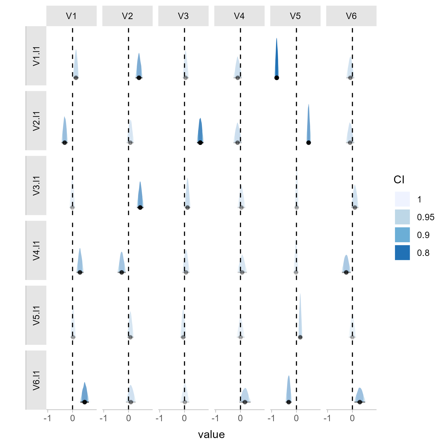

You can then compare these networks, summarize the results and plot the test results. In this case, the test is significant for both the temporal and the contemporaneous network.

# Compare networks
compare_13 <- compare_gvar(net_1, 
                           net_2,
                           return_all = TRUE,
                           n_draws = 1000)

# Print summary of results
print(compare_13)

# Plot test results
test_plot_13 <- plot(compare_13,
                     name_a = "Model A",
                     name_b = "Model B")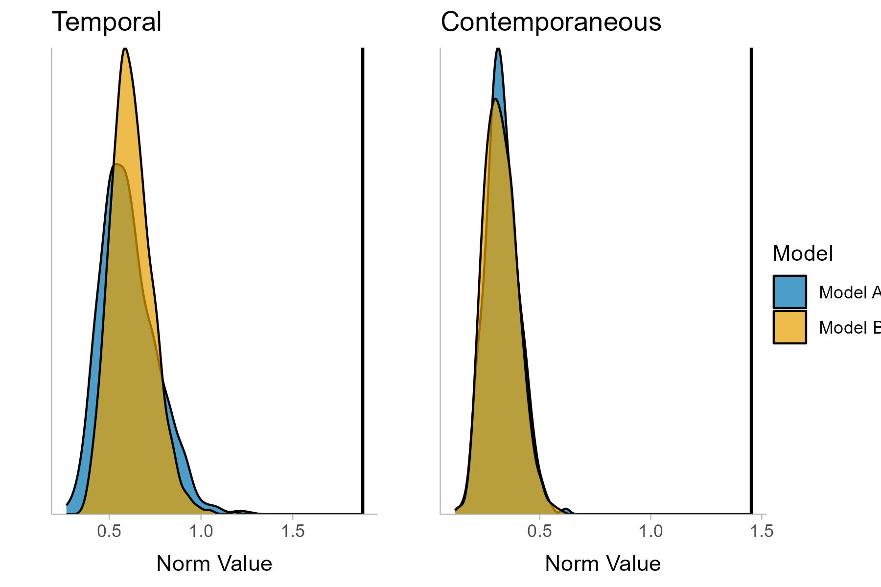

References

If you use the package, please cite the paper that introduces the package and the test:

Siepe, B. S., Kloft, M., & Heck, D. W. (2024). Bayesian estimation and comparison of idiographic network models. Psychological Methods. Advance online publication. https://doi.org/10.1037/met0000672

@article{siepe2024bayesian,
  title={Bayesian estimation and comparison of idiographic network models},
  author={Siepe, Björn S. and Kloft, Matthias and Heck, Daniel W.},
  journal={Psychological Methods},
  issue={Advance online publication},
  year={2024},
  doi={10.1037/met0000672}
}